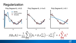
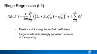
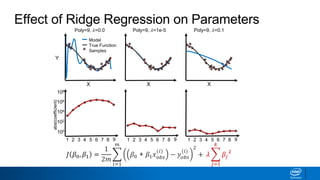
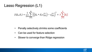
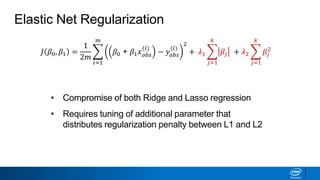
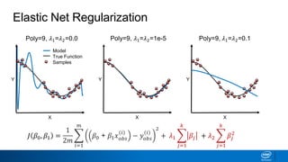
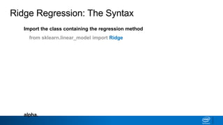
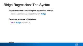
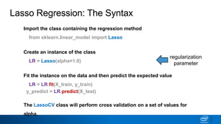
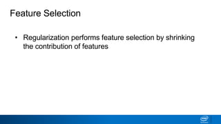
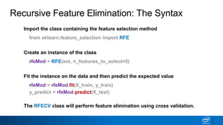
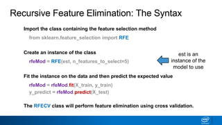
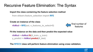
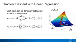
Regularization and Feature
Selection
Legal Notices and Disclaimers
This presentation is for informational purposes only. INTEL MAKES NO WARRANTIES,
EXPRESS OR IMPLIED, IN THIS SUMMARY.
Intel technologies’ features and benefits depend on system configuration and may require
enabled hardware, software or service activation. Performance varies depending on system
configuration. Check with your system manufacturer or retailer or learn more at intel.com.
This sample source code is released under the Intel Sample Source Code License Agreement.
Intel and the Intel logo are trademarks of Intel Corporation in the U.S. and/or other countries.
*Other names and brands may be claimed as the property of others.
Copyright © 2017, Intel Corporation. All rights reserved.
Model Complexity vs Error
error
𝐽𝑐𝑣 𝜃
cross validation error
𝐽𝑡𝑟𝑎𝑖𝑛 𝜃
training error
Preventing Under- and Overfitting
• How to use a degree 9 polynomial and prevent overfitting?
X
Y
Model
True Function
Samples
X
Y
X
Y
Polynomial Degree = 1 Polynomial Degree = 3 Polynomial Degree = 9
Preventing Under- and Overfitting
𝐽 𝛽0, 𝛽1 =
1
2𝑚
𝑖=1
𝑚
𝛽0 + 𝛽1 𝑥 𝑜𝑏𝑠
(𝑖)
− 𝑦𝑜𝑏𝑠
(𝑖)
2
X
Y
Model
True Function
Samples
X
Y
X
Y
Polynomial Degree = 1 Polynomial Degree = 3 Polynomial Degree = 9
Regularization
𝐽 𝛽0, 𝛽1 =
1
2𝑚
𝑖=1
𝑚
𝛽0 + 𝛽1 𝑥 𝑜𝑏𝑠
(𝑖)
− 𝑦𝑜𝑏𝑠
(𝑖)
2
+ 𝜆
𝑗=1
𝑘
𝛽𝑗
2
X
Y
Model
True Function
Samples
X
Y
X
Y
Poly Degree=9, 𝜆=0.1Poly Degree=9, 𝜆=1e-5Poly Degree=9, 𝜆=0.0
𝐽 𝛽0, 𝛽1 =
1
2𝑚
𝑖=1
𝑚
𝛽0 + 𝛽1 𝑥 𝑜𝑏𝑠
(𝑖)
− 𝑦𝑜𝑏𝑠
(𝑖)
2
+ 𝜆
𝑗=1
𝑘
𝛽𝑗
2
Ridge Regression (L2)
• Penalty shrinks magnitude of all coefficients
• Larger coefficients strongly penalized because
of the squaring
Effect of Ridge Regression on Parameters
𝐽 𝛽0, 𝛽1 =
1
2𝑚
𝑖=1
𝑚
𝛽0 + 𝛽1 𝑥 𝑜𝑏𝑠
(𝑖)
− 𝑦𝑜𝑏𝑠
(𝑖)
2
+ 𝜆
𝑗=1
𝑘
𝛽𝑗
2
X
Model
True Function
Samples
XX
Y
Poly=9, 𝜆=0.1Poly=9, 𝜆=1e-5Poly=9, 𝜆=0.0
1
abs(coefficient)
2 3 4 5 6 7 8 9 1 2 3 4 5 6 7 8 9 1 2 3 4 5 6 7 8 9
100
102
104
106
108
𝐽 𝛽0, 𝛽1 =
1
2𝑚
𝑖=1
𝑚
𝛽0 + 𝛽1 𝑥 𝑜𝑏𝑠
(𝑖)
− 𝑦𝑜𝑏𝑠
(𝑖)
2
+ 𝜆
𝑗=1
𝑘
𝛽𝑗
Lasso Regression (L1)
• Penalty selectively shrinks some coefficients
• Can be used for feature selection
• Slower to converge than Ridge regression
Effect of Lasso Regression on Parameters
𝐽 𝛽0, 𝛽1 =
1
2𝑚
𝑖=1
𝑚
𝛽0 + 𝛽1 𝑥 𝑜𝑏𝑠
(𝑖)
− 𝑦𝑜𝑏𝑠
(𝑖)
2
+ 𝜆
𝑗=1
𝑘
𝛽𝑗
X
Model
True Function
Samples
XX
Y
Poly=9, 𝜆=0.1Poly=9, 𝜆=1e-5Poly=9, 𝜆=0.0
1
abs(coefficient)
2 3 4 5 6 7 8 9 1 2 3 4 5 6 7 8 9 1 2 3 4 5 6 7 8 9
100
102
104
106
108
𝐽 𝛽0, 𝛽1 =
1
2𝑚
𝑖=1
𝑚
𝛽0 + 𝛽1 𝑥 𝑜𝑏𝑠
(𝑖)
− 𝑦𝑜𝑏𝑠
(𝑖)
2
+ 𝜆1
𝑗=1
𝑘
𝛽𝑗 + 𝜆2
𝑗=1
𝑘
𝛽𝑗
2
Elastic Net Regularization
• Compromise of both Ridge and Lasso regression
• Requires tuning of additional parameter that
distributes regularization penalty between L1 and L2
𝐽 𝛽0, 𝛽1 =
1
2𝑚
𝑖=1
𝑚
𝛽0 + 𝛽1 𝑥 𝑜𝑏𝑠
(𝑖)
− 𝑦𝑜𝑏𝑠
(𝑖)
2
+ 𝜆1
𝑗=1
𝑘
𝛽𝑗 + 𝜆2
𝑗=1
𝑘
𝛽𝑗
2
X
Y
Model
True Function
Samples
X
Y
X
Y
Poly=9, 𝜆1=𝜆2=0.1Poly=9, 𝜆1=𝜆2=1e-5Poly=9, 𝜆1=𝜆2=0.0
Elastic Net Regularization
Hyperparameters and Their Optimization
• Regularization coefficients (𝜆1 and 𝜆2)
are empirically determined
• Want value that generalizes—do not
use test data for tuning
• Create additional split of data to tune
hyperparameters—validation set
• Cross validation can also be used on
training data
Training Data
Test Data
Use Test Data to Tune 𝜆?
Hyperparameters and Their Optimization
• Regularization coefficients (𝜆1 and 𝜆2)
are empirically determined
• Want value that generalizes—do not
use test data for tuning
• Create additional split of data to tune
hyperparameters—validation set
• Cross validation can also be used on
training data
Training Data
Test Data
NO!
Use Test Data to Tune 𝜆?
Hyperparameters and Their Optimization
• Regularization coefficients (𝜆1 and 𝜆2)
are empirically determined
• Want value that generalizes—do not
use test data for tuning
• Create additional split of data to tune
hyperparameters—validation set
• Cross validation can also be used on
training data
Training Data
Test Data
Tune 𝜆 with Cross Validation
Validation
Data
Import the class containing the regression method
from sklearn.linear_model import Ridge
Create an instance of the class
RR = Ridge(alpha=1.0)
Fit the instance on the data and then predict the expected value
RR = RR.fit(X_train, y_train)
y_predict = RR.predict(X_test)
The RidgeCV class will perform cross validation on a set of values for
alpha.
Ridge Regression: The Syntax
regularization
parameter
Import the class containing the regression method
from sklearn.linear_model import Ridge
Create an instance of the class
RR = Ridge(alpha=1.0)
Fit the instance on the data and then predict the expected value
RR = RR.fit(X_train, y_train)
y_predict = RR.predict(X_test)
The RidgeCV class will perform cross validation on a set of values for
alpha.
Ridge Regression: The Syntax
Import the class containing the regression method
from sklearn.linear_model import Ridge
Create an instance of the class
RR = Ridge(alpha=1.0)
Fit the instance on the data and then predict the expected value
RR = RR.fit(X_train, y_train)
y_predict = RR.predict(X_test)
The RidgeCV class will perform cross validation on a set of values for
alpha.
Lasso Regression: The Syntax
Import the class containing the regression method
from sklearn.linear_model import Lasso
Create an instance of the class
LR = Lasso(alpha=1.0)
Fit the instance on the data and then predict the expected value
LR = LR.fit(X_train, y_train)
y_predict = LR.predict(X_test)
The LassoCV class will perform cross validation on a set of values for
alpha.
regularization
parameter
Elastic Net Regression: The Syntax
Import the class containing the regression method
from sklearn.linear_model import ElasticNet
Create an instance of the class
EN = ElasticNet(alpha=1.0, l1_ratio=0.5)
Fit the instance on the data and then predict the expected value
EN = EN.fit(X_train, y_train)
y_predict = EN.predict(X_test)
The ElasticNetCV class will perform cross validation on a set of values for
l1_ratio and alpha.
Elastic Net Regression: The Syntax
alpha is the
regularization
parameter
Import the class containing the regression method
from sklearn.linear_model import ElasticNet
Create an instance of the class
EN = ElasticNet(alpha=1.0, l1_ratio=0.5)
Fit the instance on the data and then predict the expected value
EN = EN.fit(X_train, y_train)
y_predict = EN.predict(X_test)
The ElasticNetCV class will perform cross validation on a set of values for
l1_ratio and alpha.
Elastic Net Regression: The Syntax
l1_ratio
distributes alpha
to L1/L2
Import the class containing the regression method
from sklearn.linear_model import ElasticNet
Create an instance of the class
EN = ElasticNet(alpha=1.0, l1_ratio=0.5)
Fit the instance on the data and then predict the expected value
EN = EN.fit(X_train, y_train)
y_predict = EN.predict(X_test)
The ElasticNetCV class will perform cross validation on a set of values for
l1_ratio and alpha.
Feature Selection
• Regularization performs feature selection by shrinking
the contribution of features
• For L1-regularization, this is accomplished by driving
some coefficients to zero
• Feature selection can also be performed by removing
features
Feature Selection
• Regularization performs feature selection by shrinking
the contribution of features
• For L1-regularization, this is accomplished by driving
some coefficients to zero
• Feature selection can also be performed by removing
features
Feature Selection
• Regularization performs feature selection by shrinking
the contribution of features
• For L1-regularization, this is accomplished by driving
some coefficients to zero
• Feature selection can also be performed by removing
features
Why is Feature Selection Important?
• Reducing the number of features is another way to
prevent overfitting (similar to regularization)
• For some models, fewer features can improve fitting
time and/or results
• Identifying most critical features can improve model
interpretability
Why is Feature Selection Important?
• Reducing the number of features is another way to
prevent overfitting (similar to regularization)
• For some models, fewer features can improve fitting
time and/or results
• Identifying most critical features can improve model
interpretability
Why is Feature Selection Important?
• Reducing the number of features is another way to
prevent overfitting (similar to regularization)
• For some models, fewer features can improve fitting
time and/or results
• Identifying most critical features can improve model
interpretability
Recursive Feature Elimination: The Syntax
Import the class containing the feature selection method
from sklearn.feature_selection import RFE
Create an instance of the class
rfeMod = RFE(est, n_features_to_select=5)
Fit the instance on the data and then predict the expected value
rfeMod = rfeMod.fit(X_train, y_train)
y_predict = rfeMod.predict(X_test)
The RFECV class will perform feature elimination using cross validation.
Recursive Feature Elimination: The Syntax
est is an
instance of the
model to use
Import the class containing the feature selection method
from sklearn.feature_selection import RFE
Create an instance of the class
rfeMod = RFE(est, n_features_to_select=5)
Fit the instance on the data and then predict the expected value
rfeMod = rfeMod.fit(X_train, y_train)
y_predict = rfeMod.predict(X_test)
The RFECV class will perform feature elimination using cross validation.
Recursive Feature Elimination: The Syntax
Import the class containing the feature selection method
from sklearn.feature_selection import RFE
Create an instance of the class
rfeMod = RFE(est, n_features_to_select=5)
Fit the instance on the data and then predict the expected value
rfeMod = rfeMod.fit(X_train, y_train)
y_predict = rfeMod.predict(X_test)
The RFECV class will perform feature elimination using cross validation.
final number of
features
Gradient Descent
𝐽 𝛽
Gradient Descent
𝛽
Start with a cost function J(𝛽):
Then gradually move towards the minimum.
𝐽 𝛽
Gradient Descent
𝛽
Start with a cost function J(𝛽):
Global Minimum
Gradient Descent with Linear Regression
• Now imagine there are two
parameters (𝛽0, 𝛽1)
• This is a more complicated surface
on which the minimum must be
found
• How can we do this without knowing
what 𝐽 𝛽0, 𝛽1 looks like?
𝐽 𝛽0, 𝛽1
𝛽1 𝛽0
Gradient Descent with Linear Regression
• Now imagine there are two
parameters (𝛽0, 𝛽1)
• This is a more complicated surface
on which the minimum must be
found
• How can we do this without knowing
what 𝐽 𝛽0, 𝛽1 looks like?
𝐽 𝛽0, 𝛽1
𝛽1 𝛽0
Gradient Descent with Linear Regression
• Now imagine there are two
parameters (𝛽0, 𝛽1)
• This is a more complicated surface
on which the minimum must be
found
• How can we do this without knowing
what 𝐽 𝛽0, 𝛽1 looks like?
𝐽 𝛽0, 𝛽1
𝛽1 𝛽0
• Compute the gradient, 𝛻𝐽 𝛽0, 𝛽1 , which
points in the direction of the biggest
increase!
• -𝛻𝐽 𝛽0, 𝛽1 (negative gradient) points to
the biggest decrease at that point!
𝐽 𝛽0, 𝛽1
𝛽1 𝛽0
Gradient Descent with Linear Regression
• The gradient is the a vector whose
coordinates consist of the partial
derivatives of the parameters
𝐽 𝛽0, 𝛽1
𝛽1 𝛽0
Gradient Descent with Linear Regression
𝛻𝐽 𝛽0, … , 𝛽 𝑛 = <
𝜕𝐽
𝜕𝛽0
, … ,
𝜕𝐽
𝜕𝛽 𝑛
>
• Then use the gradient (𝛻) and the cost
function to calculate the next point (𝜔1)
from the current one (𝜔0):
• The learning rate (𝛼) is a tunable
parameter that determines step size
𝐽 𝛽0, 𝛽1
𝛽1 𝛽0
Gradient Descent with Linear Regression
𝜔1 = 𝜔0 − 𝛼𝛻
1
2
𝑖=1
𝑚
𝛽0 + 𝛽1 𝑥 𝑜𝑏𝑠
(𝑖)
− 𝑦𝑜𝑏𝑠
(𝑖)
2
𝜔0
𝜔1
• Then use the gradient (𝛻) and the cost
function to calculate the next point (𝜔1)
from the current one (𝜔0):
• The learning rate (𝛼) is a tunable
parameter that determines step size
𝐽 𝛽0, 𝛽1
𝛽1 𝛽0
Gradient Descent with Linear Regression
𝜔1 = 𝜔0 − 𝛼𝛻
1
2
𝑖=1
𝑚
𝛽0 + 𝛽1 𝑥 𝑜𝑏𝑠
(𝑖)
− 𝑦𝑜𝑏𝑠
(𝑖)
2
𝜔0
𝜔1
• Each point can be iteratively calculated
from the previous one
𝐽 𝛽0, 𝛽1
𝛽1 𝛽0
Gradient Descent with Linear Regression
𝜔2 = 𝜔1 − 𝛼𝛻
1
2
𝑖=1
𝑚
𝛽0 + 𝛽1 𝑥 𝑜𝑏𝑠
(𝑖)
− 𝑦𝑜𝑏𝑠
(𝑖)
2 𝜔0
𝜔1
𝜔2
𝜔3 = 𝜔2 − 𝛼𝛻
1
2
𝑖=1
𝑚
𝛽0 + 𝛽1 𝑥 𝑜𝑏𝑠
(𝑖)
− 𝑦𝑜𝑏𝑠
(𝑖)
2
• Each point can be iteratively calculated
from the previous one
𝐽 𝛽0, 𝛽1
𝛽1 𝛽0
Gradient Descent with Linear Regression
𝜔2 = 𝜔1 − 𝛼𝛻
1
2
𝑖=1
𝑚
𝛽0 + 𝛽1 𝑥 𝑜𝑏𝑠
(𝑖)
− 𝑦𝑜𝑏𝑠
(𝑖)
2 𝜔0
𝜔1
𝜔2
𝜔3 = 𝜔2 − 𝛼𝛻
1
2
𝑖=1
𝑚
𝛽0 + 𝛽1 𝑥 𝑜𝑏𝑠
(𝑖)
− 𝑦𝑜𝑏𝑠
(𝑖)
2 𝜔3
• Use a single data point to determine the
gradient and cost function instead of all
the data
𝐽 𝛽0, 𝛽1
𝛽1 𝛽0
Stochastic Gradient Descent
𝜔1 = 𝜔0 − 𝛼𝛻
1
2
𝛽0 + 𝛽1 𝑥 𝑜𝑏𝑠
(0)
− 𝑦𝑜𝑏𝑠
(0)
2
𝜔0
𝜔1
𝜔1 = 𝜔0 − 𝛼𝛻
1
2
𝑖=1
𝑚
𝛽0 + 𝛽1 𝑥 𝑜𝑏𝑠
(𝑖)
− 𝑦𝑜𝑏𝑠
(𝑖)
2
• Use a single data point to determine the
gradient and cost function instead of all
the data
𝐽 𝛽0, 𝛽1
𝛽1 𝛽0
Stochastic Gradient Descent
𝜔0
𝜔1
𝜔1 = 𝜔0 − 𝛼𝛻
1
2
𝑖=1
𝑚
𝛽0 + 𝛽1 𝑥 𝑜𝑏𝑠
(𝑖)
− 𝑦𝑜𝑏𝑠
(𝑖)
2
• Use a single data point to determine the
gradient and cost function instead of all
the data
𝐽 𝛽0, 𝛽1
𝛽1 𝛽0
Stochastic Gradient Descent
𝜔1 = 𝜔0 − 𝛼𝛻
1
2
𝛽0 + 𝛽1 𝑥 𝑜𝑏𝑠
(0)
− 𝑦𝑜𝑏𝑠
(0)
2
𝜔0
𝜔1
𝜔1 = 𝜔0 − 𝛼𝛻
1
2
𝑖=1
𝑚
𝛽0 + 𝛽1 𝑥 𝑜𝑏𝑠
(𝑖)
− 𝑦𝑜𝑏𝑠
(𝑖)
2
𝜔4 = 𝜔3 − 𝛼𝛻
1
2
𝛽0 + 𝛽1 𝑥 𝑜𝑏𝑠
(3)
− 𝑦𝑜𝑏𝑠
(3)
2
𝐽 𝛽0, 𝛽1
𝛽1 𝛽0
Stochastic Gradient Descent
𝜔0
𝜔1
𝜔2 𝜔3 𝜔4
• Use a single data point to determine the
gradient and cost function instead of all
the data
𝜔1 = 𝜔0 − 𝛼𝛻
1
2
𝛽0 + 𝛽1 𝑥 𝑜𝑏𝑠
(0)
− 𝑦𝑜𝑏𝑠
(0)
2
…
𝜔4 = 𝜔3 − 𝛼𝛻
1
2
𝛽0 + 𝛽1 𝑥 𝑜𝑏𝑠
(3)
− 𝑦𝑜𝑏𝑠
(3)
2
𝐽 𝛽0, 𝛽1
𝛽1 𝛽0
Stochastic Gradient Descent
𝜔0
𝜔1
𝜔2 𝜔3 𝜔4
• Use a single data point to determine the
gradient and cost function instead of all
the data
• Path is less direct due to noise in single
data point—"stochastic"
𝜔1 = 𝜔0 − 𝛼𝛻
1
2
𝛽0 + 𝛽1 𝑥 𝑜𝑏𝑠
(0)
− 𝑦𝑜𝑏𝑠
(0)
2
…
• Perform an update for every 𝑛 training
examples
𝐽 𝛽0, 𝛽1
𝛽1 𝛽0
Mini Batch Gradient Descent
𝜔0
𝜔1
𝜔1 = 𝜔0 − 𝛼𝛻
1
2
𝑖=1
𝑛
𝛽0 + 𝛽1 𝑥 𝑜𝑏𝑠
(𝑖)
− 𝑦𝑜𝑏𝑠
(𝑖)
2
• Perform an update for every 𝑛 training
examples
𝐽 𝛽0, 𝛽1
𝛽1 𝛽0
Mini Batch Gradient Descent
𝜔0
𝜔1
𝜔1 = 𝜔0 − 𝛼𝛻
1
2
𝑖=1
𝑛
𝛽0 + 𝛽1 𝑥 𝑜𝑏𝑠
(𝑖)
− 𝑦𝑜𝑏𝑠
(𝑖)
2
• Perform an update for every 𝑛 training
examples
Best of both worlds:
• Reduced memory relative to "vanilla"
gradient descent
• Less noisy than stochastic gradient
descent
𝐽 𝛽0, 𝛽1
𝛽1 𝛽0
Mini Batch Gradient Descent
𝜔0
𝜔1
𝜔1 = 𝜔0 − 𝛼𝛻
1
2
𝑖=1
𝑛
𝛽0 + 𝛽1 𝑥 𝑜𝑏𝑠
(𝑖)
− 𝑦𝑜𝑏𝑠
(𝑖)
2
• Mini batch implementation typically used for neural nets
• Batch sizes range from 50-256 points
• Trade off between batch size and learning rate (α)
• Tailor learning rate schedule: gradually reduce learning rate
during a given epoch
Mini Batch Gradient Descent
• Mini batch implementation typically used for neural nets
• Batch sizes range from 50-256 points
• Trade off between batch size and learning rate (α)
• Tailor learning rate schedule: gradually reduce learning rate
during a given epoch
Mini Batch Gradient Descent
• Mini batch implementation typically used for neural nets
• Batch sizes range from 50-256 points
• Trade off between batch size and learning rate (𝛼)
• Tailor learning rate schedule: gradually reduce learning rate
during a given epoch
Mini Batch Gradient Descent
• Mini batch implementation typically used for neural nets
• Batch sizes range from 50–256 points
• Trade off between batch size and learning rate (𝛼)
• Tailor learning rate schedule: gradually reduce learning rate
during a given epoch
Mini Batch Gradient Descent
Stochastic Gradient Descent Regression: Syntax
Import the class containing the regression model
from sklearn.linear_model import SGDRegressor
Import the class containing the regression model
from sklearn.linear_model import SGDRegressor
Create an instance of the class
SGDreg = SGDRregressor(loss='squared_loss',
alpha=0.1, penalty='l2')
Stochastic Gradient Descent Regression: Syntax
Import the class containing the regression model
from sklearn.linear_model import SGDRegressor
Create an instance of the class
SGDreg = SGDRregressor(loss='squared_loss',
alpha=0.1, penalty='l2')
squared_loss =
linear
regression
Stochastic Gradient Descent Regression: Syntax
Import the class containing the regression model
from sklearn.linear_model import SGDRegressor
Create an instance of the class
SGDreg = SGDRregressor(loss='squared_loss',
alpha=0.1, penalty='l2') regularization
parameters
Stochastic Gradient Descent Regression: Syntax
Import the class containing the regression model
from sklearn.linear_model import SGDRegressor
Create an instance of the class
SGDreg = SGDRregressor(loss='squared_loss',
alpha=0.1, penalty='l2')
Fit the instance on the data and then transform the data
SGDreg = SGDreg.fit(X_train, y_train)
y_pred = SGDreg.predict(X_test)
Stochastic Gradient Descent Regression: Syntax
Import the class containing the regression model
from sklearn.linear_model import SGDRegressor
Create an instance of the class
SGDreg = SGDRregressor(loss='squared_loss',
alpha=0.1, penalty='l2')
Fit the instance on the data and then transform the data
SGDreg = SGDreg.partial_fit(X_train, y_train)
y_pred = SGDreg.predict(X_test)
Stochastic Gradient Descent Regression: Syntax
mini-batch
version
Import the class containing the regression model
from sklearn.linear_model import SGDRegressor
Create an instance of the class
SGDreg = SGDRregressor(loss='squared_loss',
alpha=0.1, penalty='l2')
Fit the instance on the data and then transform the data
SGDreg = SGDreg.fit(X_train, y_train)
y_pred = SGDreg.predict(X_test)
Other loss methods exist: epsilon_insensitive, huber, etc.
Stochastic Gradient Descent Regression: The Syntax
Import the class containing the classification model
from sklearn.linear_model import SGDClassifier
Stochastic Gradient Descent Classification: The
Syntax
Import the class containing the classification model
from sklearn.linear_model import SGDClassifier
Create an instance of the class
SGDclass = SGDClassifier(loss='log',
alpha=0.1, penalty='l2')
Stochastic Gradient Descent Classification: The
Syntax
Import the class containing the classification model
from sklearn.linear_model import SGDClassifier
Create an instance of the class
SGDclass = SGDClassifier(loss='log',
alpha=0.1, penalty='l2')
Fit the instance on the data and then transform the data
SGDclass = SGDclass.fit(X_train, y_train)
y_pred = SGDclass.predict(X_test)
Other loss methods exist: hinge, squared_hinge, etc.
log loss =
logistic regression
Stochastic Gradient Descent Classification: The
Syntax
Import the class containing the classification model
from sklearn.linear_model import SGDClassifier
Create an instance of the class
SGDclass = SGDClassifier(loss='log',
alpha=0.1, penalty='l2')
Fit the instance on the data and then transform the data
SGDclass = SGDclass.fit(X_train, y_train)
y_pred = SGDclass.predict(X_test)
Stochastic Gradient Descent Classification: The
Syntax
Import the class containing the classification model
from sklearn.linear_model import SGDClassifier
Create an instance of the class
SGDclass = SGDClassifier(loss='log',
alpha=0.1, penalty='l2')
Fit the instance on the data and then transform the data
SGDclass = SGDclass.partial_fit(X_train, y_train)
y_pred = SGDclass.predict(X_test)
Stochastic Gradient Descent Classification: The
Syntax
mini-batch
version
Import the class containing the classification model
from sklearn.linear_model import SGDClassifier
Create an instance of the class
SGDclass = SGDClassifier(loss='log',
alpha=0.1, penalty='l2')
Fit the instance on the data and then transform the data
SGDclass = SGDclass.fit(X_train, y_train)
y_pred = SGDclass.predict(X_test)
Other loss methods exist: hinge, squared_hinge, etc.
Stochastic Gradient Descent Classification: The
Syntax
Import the class containing the classification model
from sklearn.linear_model import SGDClassifier
Create an instance of the class
SGDclass = SGDClassifier(loss='log',
alpha=0.1, penalty='l2')
Fit the instance on the data and then transform the data
SGDclass = SGDclass.fit(X_train, y_train)
y_pred = SGDclass.predict(X_test)
Other loss methods exist: hinge, squared_hinge, etc.
See SVM lecture
(week 7)
Stochastic Gradient Descent Classification: The
Syntax
Ot regularization and_gradient_descent

Ot regularization and_gradient_descent

  • 1.
  • 2.
    Legal Notices andDisclaimers This presentation is for informational purposes only. INTEL MAKES NO WARRANTIES, EXPRESS OR IMPLIED, IN THIS SUMMARY. Intel technologies’ features and benefits depend on system configuration and may require enabled hardware, software or service activation. Performance varies depending on system configuration. Check with your system manufacturer or retailer or learn more at intel.com. This sample source code is released under the Intel Sample Source Code License Agreement. Intel and the Intel logo are trademarks of Intel Corporation in the U.S. and/or other countries. *Other names and brands may be claimed as the property of others. Copyright © 2017, Intel Corporation. All rights reserved.
  • 3.
    Model Complexity vsError error 𝐽𝑐𝑣 𝜃 cross validation error 𝐽𝑡𝑟𝑎𝑖𝑛 𝜃 training error
  • 4.
    Preventing Under- andOverfitting • How to use a degree 9 polynomial and prevent overfitting? X Y Model True Function Samples X Y X Y Polynomial Degree = 1 Polynomial Degree = 3 Polynomial Degree = 9
  • 5.
    Preventing Under- andOverfitting 𝐽 𝛽0, 𝛽1 = 1 2𝑚 𝑖=1 𝑚 𝛽0 + 𝛽1 𝑥 𝑜𝑏𝑠 (𝑖) − 𝑦𝑜𝑏𝑠 (𝑖) 2 X Y Model True Function Samples X Y X Y Polynomial Degree = 1 Polynomial Degree = 3 Polynomial Degree = 9
  • 6.
    Regularization 𝐽 𝛽0, 𝛽1= 1 2𝑚 𝑖=1 𝑚 𝛽0 + 𝛽1 𝑥 𝑜𝑏𝑠 (𝑖) − 𝑦𝑜𝑏𝑠 (𝑖) 2 + 𝜆 𝑗=1 𝑘 𝛽𝑗 2 X Y Model True Function Samples X Y X Y Poly Degree=9, 𝜆=0.1Poly Degree=9, 𝜆=1e-5Poly Degree=9, 𝜆=0.0
  • 7.
    𝐽 𝛽0, 𝛽1= 1 2𝑚 𝑖=1 𝑚 𝛽0 + 𝛽1 𝑥 𝑜𝑏𝑠 (𝑖) − 𝑦𝑜𝑏𝑠 (𝑖) 2 + 𝜆 𝑗=1 𝑘 𝛽𝑗 2 Ridge Regression (L2) • Penalty shrinks magnitude of all coefficients • Larger coefficients strongly penalized because of the squaring
  • 8.
    Effect of RidgeRegression on Parameters 𝐽 𝛽0, 𝛽1 = 1 2𝑚 𝑖=1 𝑚 𝛽0 + 𝛽1 𝑥 𝑜𝑏𝑠 (𝑖) − 𝑦𝑜𝑏𝑠 (𝑖) 2 + 𝜆 𝑗=1 𝑘 𝛽𝑗 2 X Model True Function Samples XX Y Poly=9, 𝜆=0.1Poly=9, 𝜆=1e-5Poly=9, 𝜆=0.0 1 abs(coefficient) 2 3 4 5 6 7 8 9 1 2 3 4 5 6 7 8 9 1 2 3 4 5 6 7 8 9 100 102 104 106 108
  • 9.
    𝐽 𝛽0, 𝛽1= 1 2𝑚 𝑖=1 𝑚 𝛽0 + 𝛽1 𝑥 𝑜𝑏𝑠 (𝑖) − 𝑦𝑜𝑏𝑠 (𝑖) 2 + 𝜆 𝑗=1 𝑘 𝛽𝑗 Lasso Regression (L1) • Penalty selectively shrinks some coefficients • Can be used for feature selection • Slower to converge than Ridge regression
  • 10.
    Effect of LassoRegression on Parameters 𝐽 𝛽0, 𝛽1 = 1 2𝑚 𝑖=1 𝑚 𝛽0 + 𝛽1 𝑥 𝑜𝑏𝑠 (𝑖) − 𝑦𝑜𝑏𝑠 (𝑖) 2 + 𝜆 𝑗=1 𝑘 𝛽𝑗 X Model True Function Samples XX Y Poly=9, 𝜆=0.1Poly=9, 𝜆=1e-5Poly=9, 𝜆=0.0 1 abs(coefficient) 2 3 4 5 6 7 8 9 1 2 3 4 5 6 7 8 9 1 2 3 4 5 6 7 8 9 100 102 104 106 108
  • 11.
    𝐽 𝛽0, 𝛽1= 1 2𝑚 𝑖=1 𝑚 𝛽0 + 𝛽1 𝑥 𝑜𝑏𝑠 (𝑖) − 𝑦𝑜𝑏𝑠 (𝑖) 2 + 𝜆1 𝑗=1 𝑘 𝛽𝑗 + 𝜆2 𝑗=1 𝑘 𝛽𝑗 2 Elastic Net Regularization • Compromise of both Ridge and Lasso regression • Requires tuning of additional parameter that distributes regularization penalty between L1 and L2
  • 12.
    𝐽 𝛽0, 𝛽1= 1 2𝑚 𝑖=1 𝑚 𝛽0 + 𝛽1 𝑥 𝑜𝑏𝑠 (𝑖) − 𝑦𝑜𝑏𝑠 (𝑖) 2 + 𝜆1 𝑗=1 𝑘 𝛽𝑗 + 𝜆2 𝑗=1 𝑘 𝛽𝑗 2 X Y Model True Function Samples X Y X Y Poly=9, 𝜆1=𝜆2=0.1Poly=9, 𝜆1=𝜆2=1e-5Poly=9, 𝜆1=𝜆2=0.0 Elastic Net Regularization
  • 13.
    Hyperparameters and TheirOptimization • Regularization coefficients (𝜆1 and 𝜆2) are empirically determined • Want value that generalizes—do not use test data for tuning • Create additional split of data to tune hyperparameters—validation set • Cross validation can also be used on training data Training Data Test Data Use Test Data to Tune 𝜆?
  • 14.
    Hyperparameters and TheirOptimization • Regularization coefficients (𝜆1 and 𝜆2) are empirically determined • Want value that generalizes—do not use test data for tuning • Create additional split of data to tune hyperparameters—validation set • Cross validation can also be used on training data Training Data Test Data NO! Use Test Data to Tune 𝜆?
  • 15.
    Hyperparameters and TheirOptimization • Regularization coefficients (𝜆1 and 𝜆2) are empirically determined • Want value that generalizes—do not use test data for tuning • Create additional split of data to tune hyperparameters—validation set • Cross validation can also be used on training data Training Data Test Data Tune 𝜆 with Cross Validation Validation Data
  • 16.
    Import the classcontaining the regression method from sklearn.linear_model import Ridge Create an instance of the class RR = Ridge(alpha=1.0) Fit the instance on the data and then predict the expected value RR = RR.fit(X_train, y_train) y_predict = RR.predict(X_test) The RidgeCV class will perform cross validation on a set of values for alpha. Ridge Regression: The Syntax
  • 17.
    Import the classcontaining the regression method from sklearn.linear_model import Ridge Create an instance of the class RR = Ridge(alpha=1.0) Fit the instance on the data and then predict the expected value RR = RR.fit(X_train, y_train) y_predict = RR.predict(X_test) The RidgeCV class will perform cross validation on a set of values for alpha. Ridge Regression: The Syntax
  • 18.
    Import the classcontaining the regression method from sklearn.linear_model import Ridge Create an instance of the class RR = Ridge(alpha=1.0) Fit the instance on the data and then predict the expected value RR = RR.fit(X_train, y_train) y_predict = RR.predict(X_test) The RidgeCV class will perform cross validation on a set of values for alpha. Ridge Regression: The Syntax regularization parameter
  • 19.
    Import the classcontaining the regression method from sklearn.linear_model import Ridge Create an instance of the class RR = Ridge(alpha=1.0) Fit the instance on the data and then predict the expected value RR = RR.fit(X_train, y_train) y_predict = RR.predict(X_test) The RidgeCV class will perform cross validation on a set of values for alpha. Ridge Regression: The Syntax
  • 20.
    Ridge Regression: TheSyntax Import the class containing the regression method from sklearn.linear_model import Ridge Create an instance of the class RR = Ridge(alpha=1.0) Fit the instance on the data and then predict the expected value RR = RR.fit(X_train, y_train) y_predict = RR.predict(X_test) The RidgeCV class will perform cross validation on a set of values for alpha.
  • 21.
    Lasso Regression: TheSyntax Import the class containing the regression method from sklearn.linear_model import Lasso Create an instance of the class LR = Lasso(alpha=1.0) Fit the instance on the data and then predict the expected value LR = LR.fit(X_train, y_train) y_predict = LR.predict(X_test) The LassoCV class will perform cross validation on a set of values for alpha.
  • 22.
    Lasso Regression: TheSyntax Import the class containing the regression method from sklearn.linear_model import Lasso Create an instance of the class LR = Lasso(alpha=1.0) Fit the instance on the data and then predict the expected value LR = LR.fit(X_train, y_train) y_predict = LR.predict(X_test) The LassoCV class will perform cross validation on a set of values for alpha. regularization parameter
  • 23.
    Elastic Net Regression:The Syntax Import the class containing the regression method from sklearn.linear_model import ElasticNet Create an instance of the class EN = ElasticNet(alpha=1.0, l1_ratio=0.5) Fit the instance on the data and then predict the expected value EN = EN.fit(X_train, y_train) y_predict = EN.predict(X_test) The ElasticNetCV class will perform cross validation on a set of values for l1_ratio and alpha.
  • 24.
    Elastic Net Regression:The Syntax alpha is the regularization parameter Import the class containing the regression method from sklearn.linear_model import ElasticNet Create an instance of the class EN = ElasticNet(alpha=1.0, l1_ratio=0.5) Fit the instance on the data and then predict the expected value EN = EN.fit(X_train, y_train) y_predict = EN.predict(X_test) The ElasticNetCV class will perform cross validation on a set of values for l1_ratio and alpha.
  • 25.
    Elastic Net Regression:The Syntax l1_ratio distributes alpha to L1/L2 Import the class containing the regression method from sklearn.linear_model import ElasticNet Create an instance of the class EN = ElasticNet(alpha=1.0, l1_ratio=0.5) Fit the instance on the data and then predict the expected value EN = EN.fit(X_train, y_train) y_predict = EN.predict(X_test) The ElasticNetCV class will perform cross validation on a set of values for l1_ratio and alpha.
  • 26.
    Feature Selection • Regularizationperforms feature selection by shrinking the contribution of features • For L1-regularization, this is accomplished by driving some coefficients to zero • Feature selection can also be performed by removing features
  • 27.
    Feature Selection • Regularizationperforms feature selection by shrinking the contribution of features • For L1-regularization, this is accomplished by driving some coefficients to zero • Feature selection can also be performed by removing features
  • 28.
    Feature Selection • Regularizationperforms feature selection by shrinking the contribution of features • For L1-regularization, this is accomplished by driving some coefficients to zero • Feature selection can also be performed by removing features
  • 29.
    Why is FeatureSelection Important? • Reducing the number of features is another way to prevent overfitting (similar to regularization) • For some models, fewer features can improve fitting time and/or results • Identifying most critical features can improve model interpretability
  • 30.
    Why is FeatureSelection Important? • Reducing the number of features is another way to prevent overfitting (similar to regularization) • For some models, fewer features can improve fitting time and/or results • Identifying most critical features can improve model interpretability
  • 31.
    Why is FeatureSelection Important? • Reducing the number of features is another way to prevent overfitting (similar to regularization) • For some models, fewer features can improve fitting time and/or results • Identifying most critical features can improve model interpretability
  • 32.
    Recursive Feature Elimination:The Syntax Import the class containing the feature selection method from sklearn.feature_selection import RFE Create an instance of the class rfeMod = RFE(est, n_features_to_select=5) Fit the instance on the data and then predict the expected value rfeMod = rfeMod.fit(X_train, y_train) y_predict = rfeMod.predict(X_test) The RFECV class will perform feature elimination using cross validation.
  • 33.
    Recursive Feature Elimination:The Syntax est is an instance of the model to use Import the class containing the feature selection method from sklearn.feature_selection import RFE Create an instance of the class rfeMod = RFE(est, n_features_to_select=5) Fit the instance on the data and then predict the expected value rfeMod = rfeMod.fit(X_train, y_train) y_predict = rfeMod.predict(X_test) The RFECV class will perform feature elimination using cross validation.
  • 34.
    Recursive Feature Elimination:The Syntax Import the class containing the feature selection method from sklearn.feature_selection import RFE Create an instance of the class rfeMod = RFE(est, n_features_to_select=5) Fit the instance on the data and then predict the expected value rfeMod = rfeMod.fit(X_train, y_train) y_predict = rfeMod.predict(X_test) The RFECV class will perform feature elimination using cross validation. final number of features
  • 36.
  • 37.
    𝐽 𝛽 Gradient Descent 𝛽 Startwith a cost function J(𝛽):
  • 38.
    Then gradually movetowards the minimum. 𝐽 𝛽 Gradient Descent 𝛽 Start with a cost function J(𝛽): Global Minimum
  • 39.
    Gradient Descent withLinear Regression • Now imagine there are two parameters (𝛽0, 𝛽1) • This is a more complicated surface on which the minimum must be found • How can we do this without knowing what 𝐽 𝛽0, 𝛽1 looks like? 𝐽 𝛽0, 𝛽1 𝛽1 𝛽0
  • 40.
    Gradient Descent withLinear Regression • Now imagine there are two parameters (𝛽0, 𝛽1) • This is a more complicated surface on which the minimum must be found • How can we do this without knowing what 𝐽 𝛽0, 𝛽1 looks like? 𝐽 𝛽0, 𝛽1 𝛽1 𝛽0
  • 41.
    Gradient Descent withLinear Regression • Now imagine there are two parameters (𝛽0, 𝛽1) • This is a more complicated surface on which the minimum must be found • How can we do this without knowing what 𝐽 𝛽0, 𝛽1 looks like? 𝐽 𝛽0, 𝛽1 𝛽1 𝛽0
  • 42.
    • Compute thegradient, 𝛻𝐽 𝛽0, 𝛽1 , which points in the direction of the biggest increase! • -𝛻𝐽 𝛽0, 𝛽1 (negative gradient) points to the biggest decrease at that point! 𝐽 𝛽0, 𝛽1 𝛽1 𝛽0 Gradient Descent with Linear Regression
  • 43.
    • The gradientis the a vector whose coordinates consist of the partial derivatives of the parameters 𝐽 𝛽0, 𝛽1 𝛽1 𝛽0 Gradient Descent with Linear Regression 𝛻𝐽 𝛽0, … , 𝛽 𝑛 = < 𝜕𝐽 𝜕𝛽0 , … , 𝜕𝐽 𝜕𝛽 𝑛 >
  • 44.
    • Then usethe gradient (𝛻) and the cost function to calculate the next point (𝜔1) from the current one (𝜔0): • The learning rate (𝛼) is a tunable parameter that determines step size 𝐽 𝛽0, 𝛽1 𝛽1 𝛽0 Gradient Descent with Linear Regression 𝜔1 = 𝜔0 − 𝛼𝛻 1 2 𝑖=1 𝑚 𝛽0 + 𝛽1 𝑥 𝑜𝑏𝑠 (𝑖) − 𝑦𝑜𝑏𝑠 (𝑖) 2 𝜔0 𝜔1
  • 45.
    • Then usethe gradient (𝛻) and the cost function to calculate the next point (𝜔1) from the current one (𝜔0): • The learning rate (𝛼) is a tunable parameter that determines step size 𝐽 𝛽0, 𝛽1 𝛽1 𝛽0 Gradient Descent with Linear Regression 𝜔1 = 𝜔0 − 𝛼𝛻 1 2 𝑖=1 𝑚 𝛽0 + 𝛽1 𝑥 𝑜𝑏𝑠 (𝑖) − 𝑦𝑜𝑏𝑠 (𝑖) 2 𝜔0 𝜔1
  • 46.
    • Each pointcan be iteratively calculated from the previous one 𝐽 𝛽0, 𝛽1 𝛽1 𝛽0 Gradient Descent with Linear Regression 𝜔2 = 𝜔1 − 𝛼𝛻 1 2 𝑖=1 𝑚 𝛽0 + 𝛽1 𝑥 𝑜𝑏𝑠 (𝑖) − 𝑦𝑜𝑏𝑠 (𝑖) 2 𝜔0 𝜔1 𝜔2 𝜔3 = 𝜔2 − 𝛼𝛻 1 2 𝑖=1 𝑚 𝛽0 + 𝛽1 𝑥 𝑜𝑏𝑠 (𝑖) − 𝑦𝑜𝑏𝑠 (𝑖) 2
  • 47.
    • Each pointcan be iteratively calculated from the previous one 𝐽 𝛽0, 𝛽1 𝛽1 𝛽0 Gradient Descent with Linear Regression 𝜔2 = 𝜔1 − 𝛼𝛻 1 2 𝑖=1 𝑚 𝛽0 + 𝛽1 𝑥 𝑜𝑏𝑠 (𝑖) − 𝑦𝑜𝑏𝑠 (𝑖) 2 𝜔0 𝜔1 𝜔2 𝜔3 = 𝜔2 − 𝛼𝛻 1 2 𝑖=1 𝑚 𝛽0 + 𝛽1 𝑥 𝑜𝑏𝑠 (𝑖) − 𝑦𝑜𝑏𝑠 (𝑖) 2 𝜔3
  • 48.
    • Use asingle data point to determine the gradient and cost function instead of all the data 𝐽 𝛽0, 𝛽1 𝛽1 𝛽0 Stochastic Gradient Descent 𝜔1 = 𝜔0 − 𝛼𝛻 1 2 𝛽0 + 𝛽1 𝑥 𝑜𝑏𝑠 (0) − 𝑦𝑜𝑏𝑠 (0) 2 𝜔0 𝜔1 𝜔1 = 𝜔0 − 𝛼𝛻 1 2 𝑖=1 𝑚 𝛽0 + 𝛽1 𝑥 𝑜𝑏𝑠 (𝑖) − 𝑦𝑜𝑏𝑠 (𝑖) 2
  • 49.
    • Use asingle data point to determine the gradient and cost function instead of all the data 𝐽 𝛽0, 𝛽1 𝛽1 𝛽0 Stochastic Gradient Descent 𝜔0 𝜔1 𝜔1 = 𝜔0 − 𝛼𝛻 1 2 𝑖=1 𝑚 𝛽0 + 𝛽1 𝑥 𝑜𝑏𝑠 (𝑖) − 𝑦𝑜𝑏𝑠 (𝑖) 2
  • 50.
    • Use asingle data point to determine the gradient and cost function instead of all the data 𝐽 𝛽0, 𝛽1 𝛽1 𝛽0 Stochastic Gradient Descent 𝜔1 = 𝜔0 − 𝛼𝛻 1 2 𝛽0 + 𝛽1 𝑥 𝑜𝑏𝑠 (0) − 𝑦𝑜𝑏𝑠 (0) 2 𝜔0 𝜔1 𝜔1 = 𝜔0 − 𝛼𝛻 1 2 𝑖=1 𝑚 𝛽0 + 𝛽1 𝑥 𝑜𝑏𝑠 (𝑖) − 𝑦𝑜𝑏𝑠 (𝑖) 2
  • 51.
    𝜔4 = 𝜔3− 𝛼𝛻 1 2 𝛽0 + 𝛽1 𝑥 𝑜𝑏𝑠 (3) − 𝑦𝑜𝑏𝑠 (3) 2 𝐽 𝛽0, 𝛽1 𝛽1 𝛽0 Stochastic Gradient Descent 𝜔0 𝜔1 𝜔2 𝜔3 𝜔4 • Use a single data point to determine the gradient and cost function instead of all the data 𝜔1 = 𝜔0 − 𝛼𝛻 1 2 𝛽0 + 𝛽1 𝑥 𝑜𝑏𝑠 (0) − 𝑦𝑜𝑏𝑠 (0) 2 …
  • 52.
    𝜔4 = 𝜔3− 𝛼𝛻 1 2 𝛽0 + 𝛽1 𝑥 𝑜𝑏𝑠 (3) − 𝑦𝑜𝑏𝑠 (3) 2 𝐽 𝛽0, 𝛽1 𝛽1 𝛽0 Stochastic Gradient Descent 𝜔0 𝜔1 𝜔2 𝜔3 𝜔4 • Use a single data point to determine the gradient and cost function instead of all the data • Path is less direct due to noise in single data point—"stochastic" 𝜔1 = 𝜔0 − 𝛼𝛻 1 2 𝛽0 + 𝛽1 𝑥 𝑜𝑏𝑠 (0) − 𝑦𝑜𝑏𝑠 (0) 2 …
  • 53.
    • Perform anupdate for every 𝑛 training examples 𝐽 𝛽0, 𝛽1 𝛽1 𝛽0 Mini Batch Gradient Descent 𝜔0 𝜔1 𝜔1 = 𝜔0 − 𝛼𝛻 1 2 𝑖=1 𝑛 𝛽0 + 𝛽1 𝑥 𝑜𝑏𝑠 (𝑖) − 𝑦𝑜𝑏𝑠 (𝑖) 2
  • 54.
    • Perform anupdate for every 𝑛 training examples 𝐽 𝛽0, 𝛽1 𝛽1 𝛽0 Mini Batch Gradient Descent 𝜔0 𝜔1 𝜔1 = 𝜔0 − 𝛼𝛻 1 2 𝑖=1 𝑛 𝛽0 + 𝛽1 𝑥 𝑜𝑏𝑠 (𝑖) − 𝑦𝑜𝑏𝑠 (𝑖) 2
  • 55.
    • Perform anupdate for every 𝑛 training examples Best of both worlds: • Reduced memory relative to "vanilla" gradient descent • Less noisy than stochastic gradient descent 𝐽 𝛽0, 𝛽1 𝛽1 𝛽0 Mini Batch Gradient Descent 𝜔0 𝜔1 𝜔1 = 𝜔0 − 𝛼𝛻 1 2 𝑖=1 𝑛 𝛽0 + 𝛽1 𝑥 𝑜𝑏𝑠 (𝑖) − 𝑦𝑜𝑏𝑠 (𝑖) 2
  • 56.
    • Mini batchimplementation typically used for neural nets • Batch sizes range from 50-256 points • Trade off between batch size and learning rate (α) • Tailor learning rate schedule: gradually reduce learning rate during a given epoch Mini Batch Gradient Descent
  • 57.
    • Mini batchimplementation typically used for neural nets • Batch sizes range from 50-256 points • Trade off between batch size and learning rate (α) • Tailor learning rate schedule: gradually reduce learning rate during a given epoch Mini Batch Gradient Descent
  • 58.
    • Mini batchimplementation typically used for neural nets • Batch sizes range from 50-256 points • Trade off between batch size and learning rate (𝛼) • Tailor learning rate schedule: gradually reduce learning rate during a given epoch Mini Batch Gradient Descent
  • 59.
    • Mini batchimplementation typically used for neural nets • Batch sizes range from 50–256 points • Trade off between batch size and learning rate (𝛼) • Tailor learning rate schedule: gradually reduce learning rate during a given epoch Mini Batch Gradient Descent
  • 60.
    Stochastic Gradient DescentRegression: Syntax Import the class containing the regression model from sklearn.linear_model import SGDRegressor
  • 61.
    Import the classcontaining the regression model from sklearn.linear_model import SGDRegressor Create an instance of the class SGDreg = SGDRregressor(loss='squared_loss', alpha=0.1, penalty='l2') Stochastic Gradient Descent Regression: Syntax
  • 62.
    Import the classcontaining the regression model from sklearn.linear_model import SGDRegressor Create an instance of the class SGDreg = SGDRregressor(loss='squared_loss', alpha=0.1, penalty='l2') squared_loss = linear regression Stochastic Gradient Descent Regression: Syntax
  • 63.
    Import the classcontaining the regression model from sklearn.linear_model import SGDRegressor Create an instance of the class SGDreg = SGDRregressor(loss='squared_loss', alpha=0.1, penalty='l2') regularization parameters Stochastic Gradient Descent Regression: Syntax
  • 64.
    Import the classcontaining the regression model from sklearn.linear_model import SGDRegressor Create an instance of the class SGDreg = SGDRregressor(loss='squared_loss', alpha=0.1, penalty='l2') Fit the instance on the data and then transform the data SGDreg = SGDreg.fit(X_train, y_train) y_pred = SGDreg.predict(X_test) Stochastic Gradient Descent Regression: Syntax
  • 65.
    Import the classcontaining the regression model from sklearn.linear_model import SGDRegressor Create an instance of the class SGDreg = SGDRregressor(loss='squared_loss', alpha=0.1, penalty='l2') Fit the instance on the data and then transform the data SGDreg = SGDreg.partial_fit(X_train, y_train) y_pred = SGDreg.predict(X_test) Stochastic Gradient Descent Regression: Syntax mini-batch version
  • 66.
    Import the classcontaining the regression model from sklearn.linear_model import SGDRegressor Create an instance of the class SGDreg = SGDRregressor(loss='squared_loss', alpha=0.1, penalty='l2') Fit the instance on the data and then transform the data SGDreg = SGDreg.fit(X_train, y_train) y_pred = SGDreg.predict(X_test) Other loss methods exist: epsilon_insensitive, huber, etc. Stochastic Gradient Descent Regression: The Syntax
  • 67.
    Import the classcontaining the classification model from sklearn.linear_model import SGDClassifier Stochastic Gradient Descent Classification: The Syntax
  • 68.
    Import the classcontaining the classification model from sklearn.linear_model import SGDClassifier Create an instance of the class SGDclass = SGDClassifier(loss='log', alpha=0.1, penalty='l2') Stochastic Gradient Descent Classification: The Syntax
  • 69.
    Import the classcontaining the classification model from sklearn.linear_model import SGDClassifier Create an instance of the class SGDclass = SGDClassifier(loss='log', alpha=0.1, penalty='l2') Fit the instance on the data and then transform the data SGDclass = SGDclass.fit(X_train, y_train) y_pred = SGDclass.predict(X_test) Other loss methods exist: hinge, squared_hinge, etc. log loss = logistic regression Stochastic Gradient Descent Classification: The Syntax
  • 70.
    Import the classcontaining the classification model from sklearn.linear_model import SGDClassifier Create an instance of the class SGDclass = SGDClassifier(loss='log', alpha=0.1, penalty='l2') Fit the instance on the data and then transform the data SGDclass = SGDclass.fit(X_train, y_train) y_pred = SGDclass.predict(X_test) Stochastic Gradient Descent Classification: The Syntax
  • 71.
    Import the classcontaining the classification model from sklearn.linear_model import SGDClassifier Create an instance of the class SGDclass = SGDClassifier(loss='log', alpha=0.1, penalty='l2') Fit the instance on the data and then transform the data SGDclass = SGDclass.partial_fit(X_train, y_train) y_pred = SGDclass.predict(X_test) Stochastic Gradient Descent Classification: The Syntax mini-batch version
  • 72.
    Import the classcontaining the classification model from sklearn.linear_model import SGDClassifier Create an instance of the class SGDclass = SGDClassifier(loss='log', alpha=0.1, penalty='l2') Fit the instance on the data and then transform the data SGDclass = SGDclass.fit(X_train, y_train) y_pred = SGDclass.predict(X_test) Other loss methods exist: hinge, squared_hinge, etc. Stochastic Gradient Descent Classification: The Syntax
  • 73.
    Import the classcontaining the classification model from sklearn.linear_model import SGDClassifier Create an instance of the class SGDclass = SGDClassifier(loss='log', alpha=0.1, penalty='l2') Fit the instance on the data and then transform the data SGDclass = SGDclass.fit(X_train, y_train) y_pred = SGDclass.predict(X_test) Other loss methods exist: hinge, squared_hinge, etc. See SVM lecture (week 7) Stochastic Gradient Descent Classification: The Syntax