
![Binary Logistic Regression – Cost Function
Cost for a single data point is known as the Loss
Take the Loss Function of Logistic Regression as L{f(X)}
L f X , Y = ቊ
− log f(X) if Y = 1
− log 1 − f(X) if Y = 0
L f X , Y = −Y log f(X) −(1 − Y) log 1 − f(X)
Cost function: J(β) =
1
n
σ𝑖=1
n
L f x , Y
J(β) =
1
n
𝑖=1
n
[−Y log f(X) − (1 − Y) log 1 − f(X) ]
This Cost Function is Convex (has a Global Minimum)](https://image.slidesharecdn.com/lec6-240412205500-3921a10c/85/Lecture-6-Logistic-Regression-a-lecture-in-subject-module-Statistical-Machine-Learning-15-320.jpg)
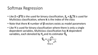
![Softmax Regression
Loss function:
L f X , Y = -log(
Yk) = -log(
eZ𝑘
j=1
K
e
Zj
) = -log(
eβk
TX
j=1
K
e
βj
TX
)
Cost function (Cross Entropy Loss):
J(β) = − ා
𝑖=1
N
Σk=1
K
I[Yi = k]log(
eβk
TX
j=1
K
e
βj
TX
)](https://image.slidesharecdn.com/lec6-240412205500-3921a10c/85/Lecture-6-Logistic-Regression-a-lecture-in-subject-module-Statistical-Machine-Learning-21-320.jpg)


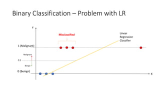
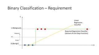
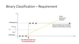
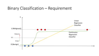
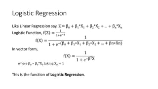
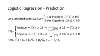
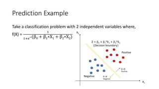
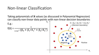
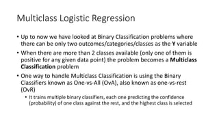
The document covers logistic regression, a statistical method used for classification problems where the dependent variable consists of distinct classes. It details binary classification with examples, discusses the sigmoid function as a continuous alternative to the unit step function, and introduces multiclass logistic regression techniques like one-vs-all and softmax classifiers. The document also addresses cost functions and emphasizes the foundational role of logistic regression in deep neural networks.