SlideShare a Scribd company logo
1 of 52
Part II
Legal Notices and Disclaimers
This presentation is for informational purposes only. INTEL MAKES NO WARRANTIES,
EXPRESS OR IMPLIED, IN THIS SUMMARY.
Intel technologies’ features and benefits depend on system configuration and may require
enabled hardware, software or service activation. Performance varies depending on system
configuration. Check with your system manufacturer or retailer or learn more at intel.com.
This sample source code is released under the Intel Sample Source Code License
Agreement.
Intel and the Intel logo are trademarks of Intel Corporation in the U.S. and/or other countries.
*Other names and brands may be claimed as the property of others.
Copyright Β© 2018, Intel Corporation. All rights reserved.
2
Canny Edge Detection
This algorithm performs edge detection by completing the following steps:
1. Remove noise with a 5x5 Gaussian
2. Detect horizontal and vertical edges
 The x,y gradients are first computed and then combined into four directional
derivatives
3. Suppress non-maximums (in direction of gradient)
Local maxima define edges
Canny Edge Detection Continued…
4. Apply two thresholds, high and low
Points below low are dropped
Points above high are kept
Points in between are kept if they connect to a kept point
High: Low thresholds should be between 2:1 and 3:1
Note: Direction of gradient is perpendicular to direction of edge
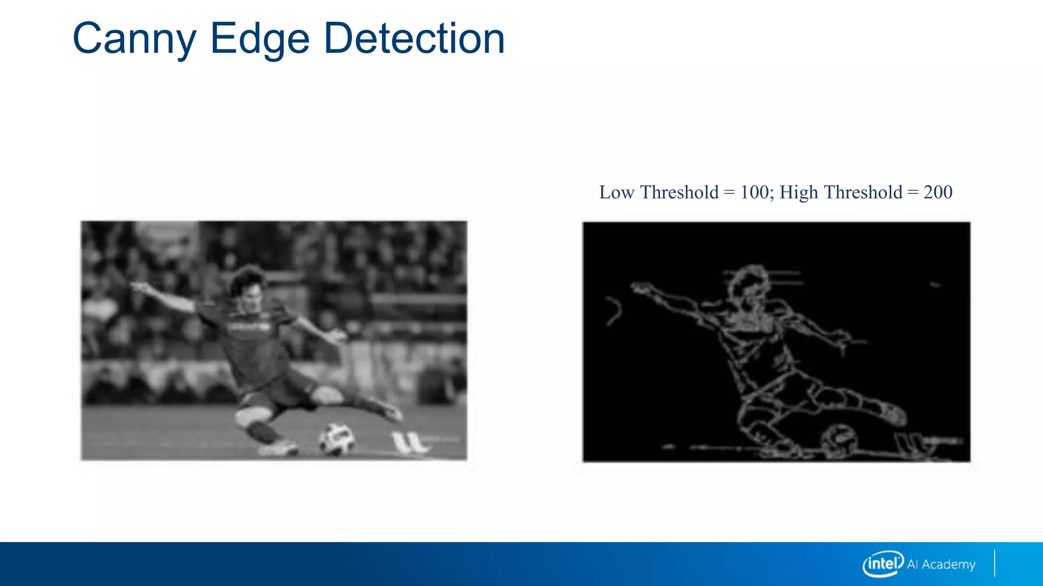
Canny Edge Detection
Low Threshold = 100; High Threshold = 200
Ptolemy and Complex Representation of
Planet Motions
Ptolemy and the ancients had a model of the planets:
β€’ Deferents and epicycles
β€’ A series of smaller circles turning on bigger circles
This modeled the observed motions of the planets fairly well
Ptolemy and Complex Representation of
Planet Motions
But the model was not explanatory.
Why? (CLICK ME)
An infinite sum of circles on top of circles can trace ANY fairly well-behaved (continuous
and not too wiggly) path ...
This is the fundamental idea of Fourier methods.
https://www.youtube.com/watch?v=QVuU2YCwHjw
Ptolemy and Complex Representation of
Planet Motions
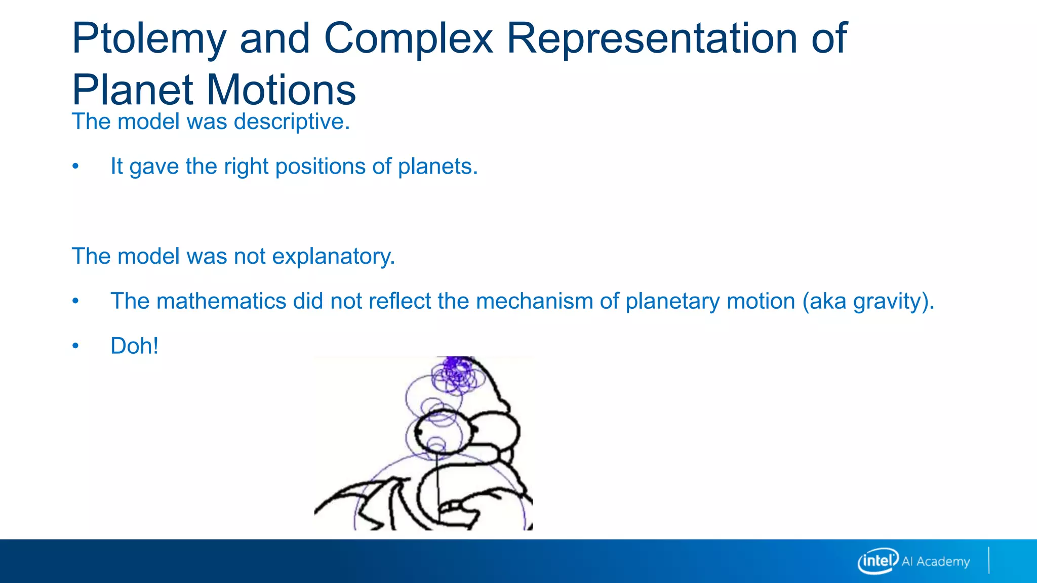
The model was descriptive.
β€’ It gave the right positions of planets.
The model was not explanatory.
β€’ The mathematics did not reflect the mechanism of planetary motion (aka gravity).
β€’ Doh!
Fourier Techniques
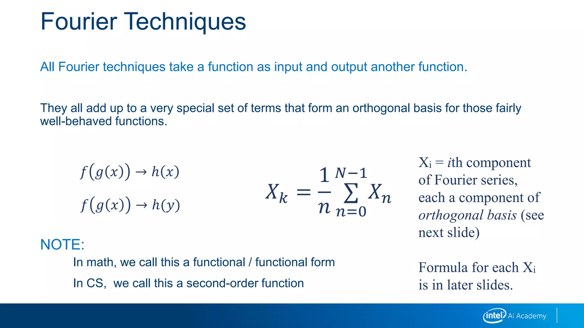
All Fourier techniques take a function as input and output another function.
They all add up to a very special set of terms that form an orthogonal basis for those fairly
well-behaved functions.
NOTE:
In math, we call this a functional / functional form
In CS, we call this a second-order function
𝑓 𝑔 π‘₯ β†’ β„Ž π‘₯
𝑓 𝑔 π‘₯ β†’ β„Ž(𝑦)
𝑋 π‘˜ =
1
𝑛
βˆ‘
𝑛=0
π‘βˆ’1
𝑋 𝑛
Xi = ith component
of Fourier series,
each a component of
orthogonal basis (see
next slide)
Formula for each Xi
is in later slides.
Fourier Techniques
Orthogonal? Basis?
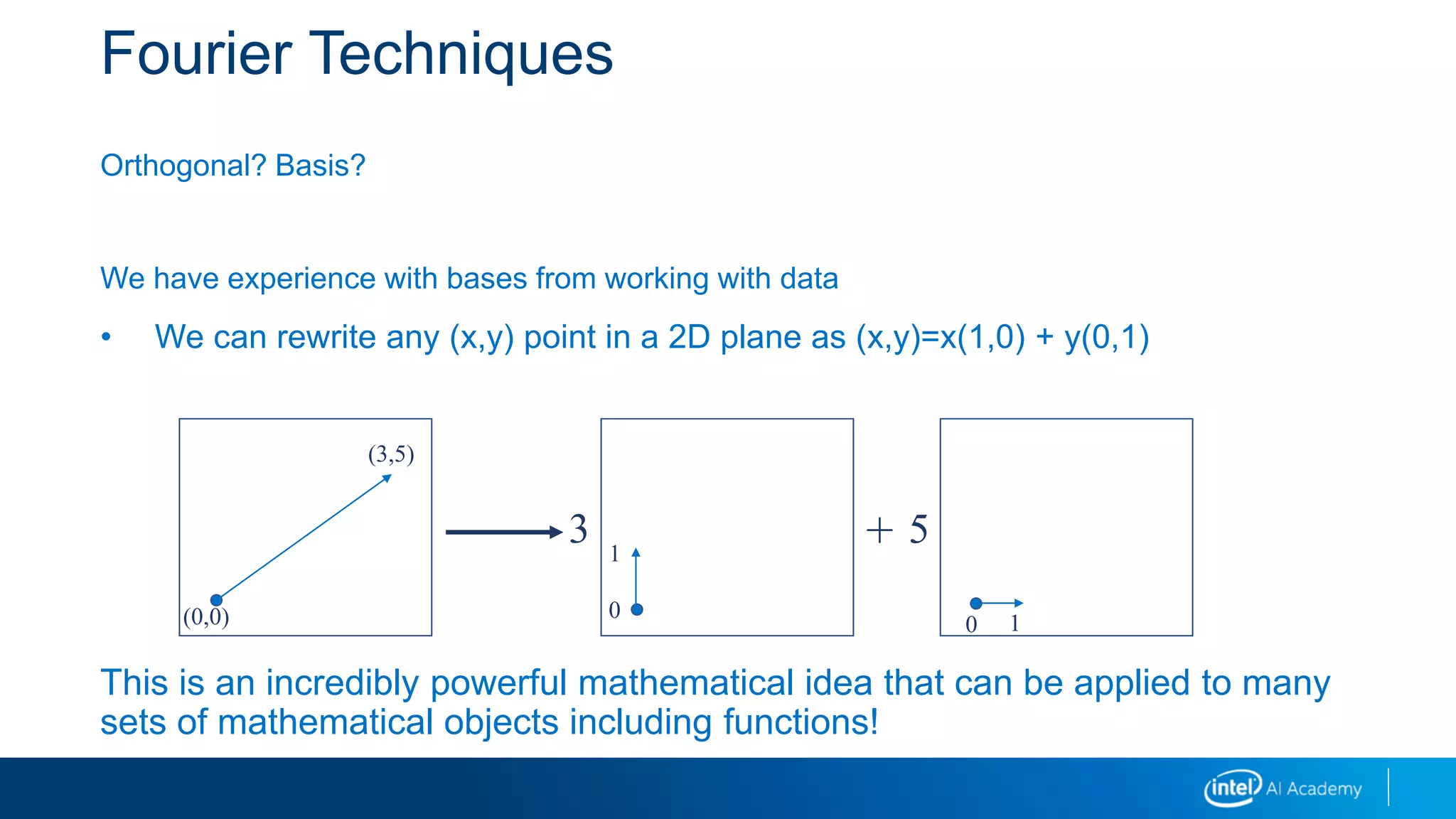
We have experience with bases from working with data
β€’ We can rewrite any (x,y) point in a 2D plane as (x,y)=x(1,0) + y(0,1)
This is an incredibly powerful mathematical idea that can be applied to many
sets of mathematical objects including functions!
(0,0)
(3,5)
3
0
1
5
0 1
+
How Does Fourier Work?
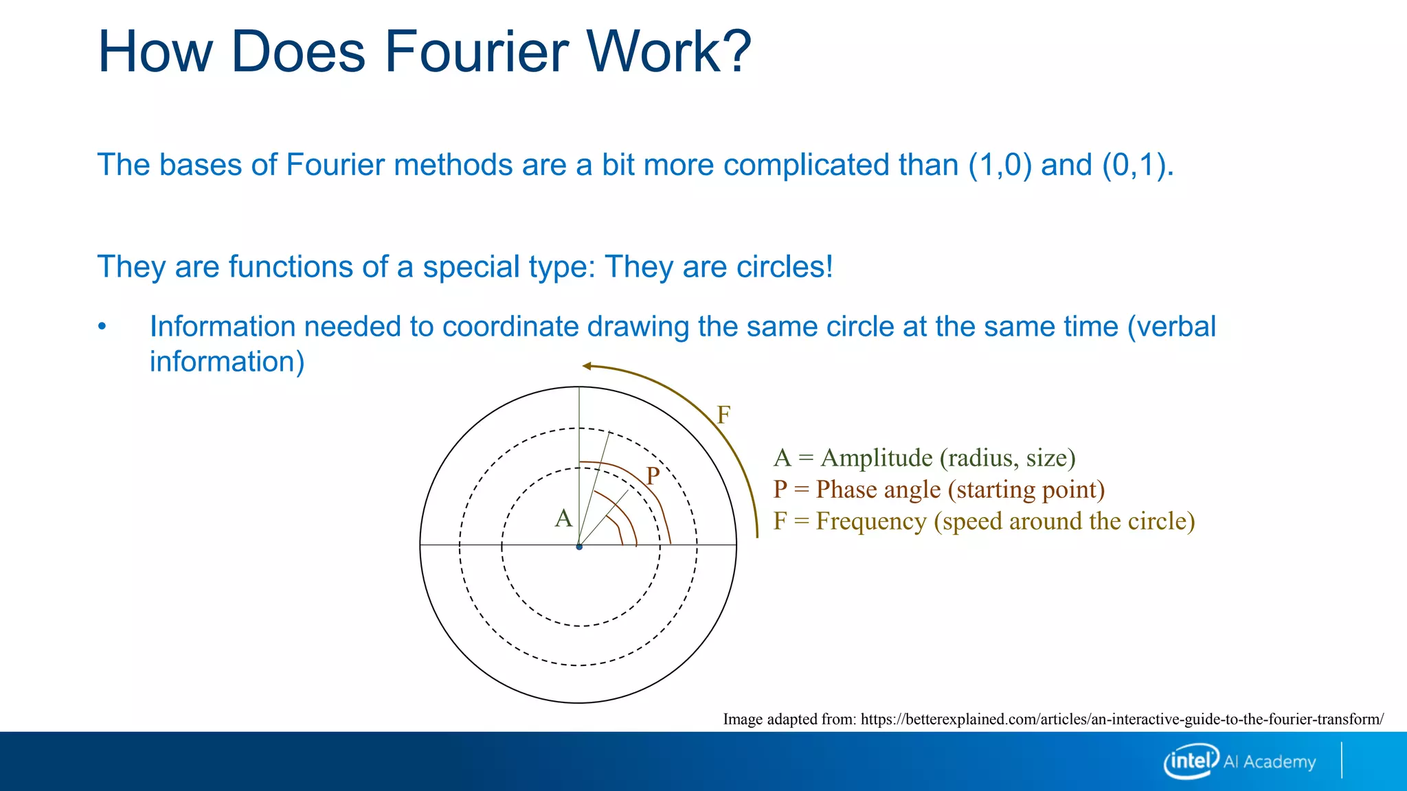
The bases of Fourier methods are a bit more complicated than (1,0) and (0,1).
They are functions of a special type: They are circles!
β€’ Information needed to coordinate drawing the same circle at the same time (verbal
information)
Image adapted from: https://betterexplained.com/articles/an-interactive-guide-to-the-fourier-transform/
A = Amplitude (radius, size)
P = Phase angle (starting point)
F = Frequency (speed around the circle)A
P
F
Fourier Methods
Fourier methods rewrite a function f in terms of an infinite sum of circles.
The rewritten function is defined at a different set of inputs and produces different
outputs:
β€’ Inputs: Frequencies (speeds of drawing the circles)
β€’ Outputs: The radii and phases (size of circle and angle of starting point)
How Does Fourier Work?
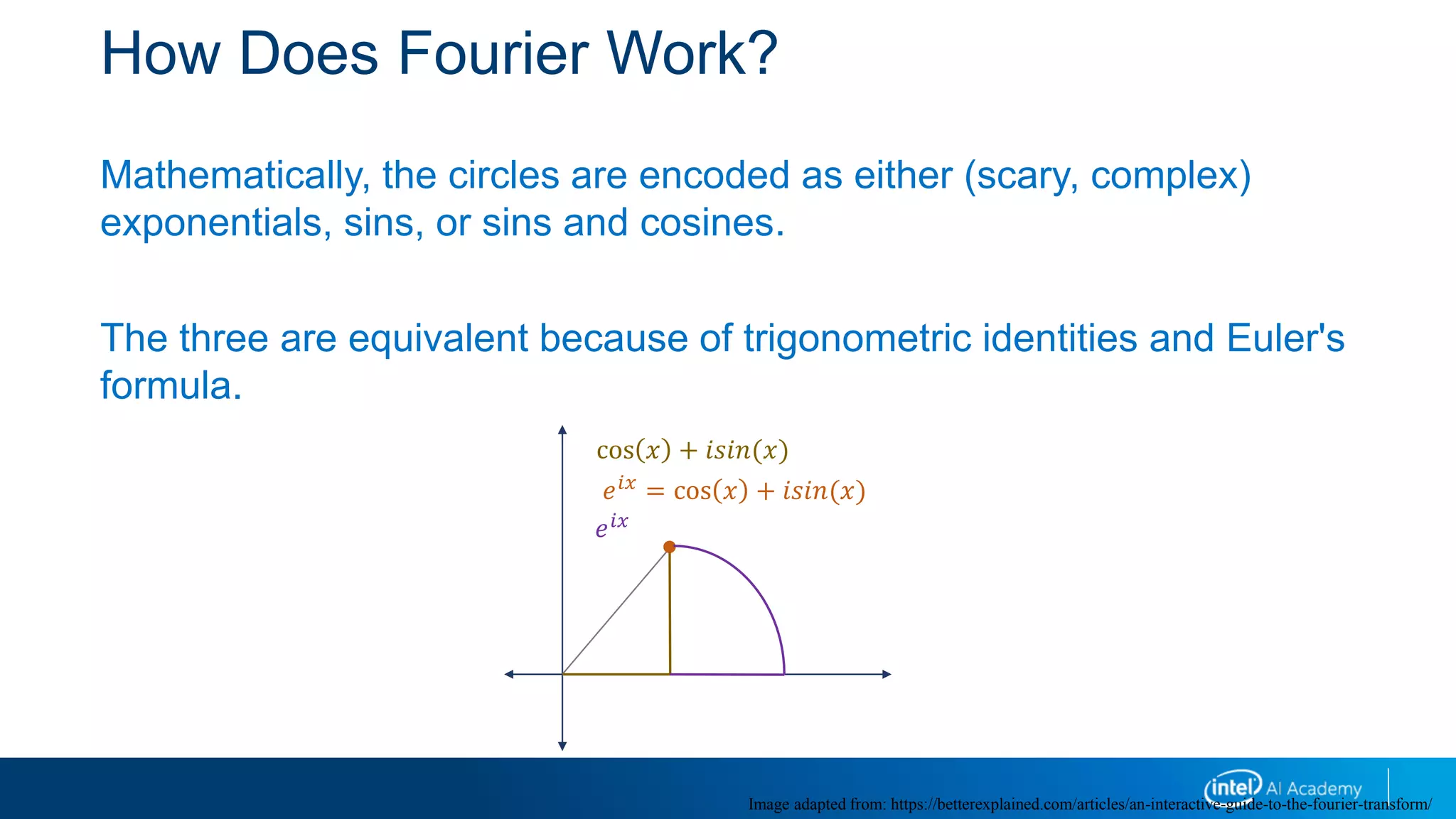
Mathematically, the circles are encoded as either (scary, complex)
exponentials, sins, or sins and cosines.
The three are equivalent because of trigonometric identities and Euler's
formula.
Image adapted from: https://betterexplained.com/articles/an-interactive-guide-to-the-fourier-transform/
cos π‘₯ + 𝑖𝑠𝑖𝑛(π‘₯)
𝑒 𝑖π‘₯ = cos π‘₯ + 𝑖𝑠𝑖𝑛(π‘₯)
𝑒 𝑖π‘₯
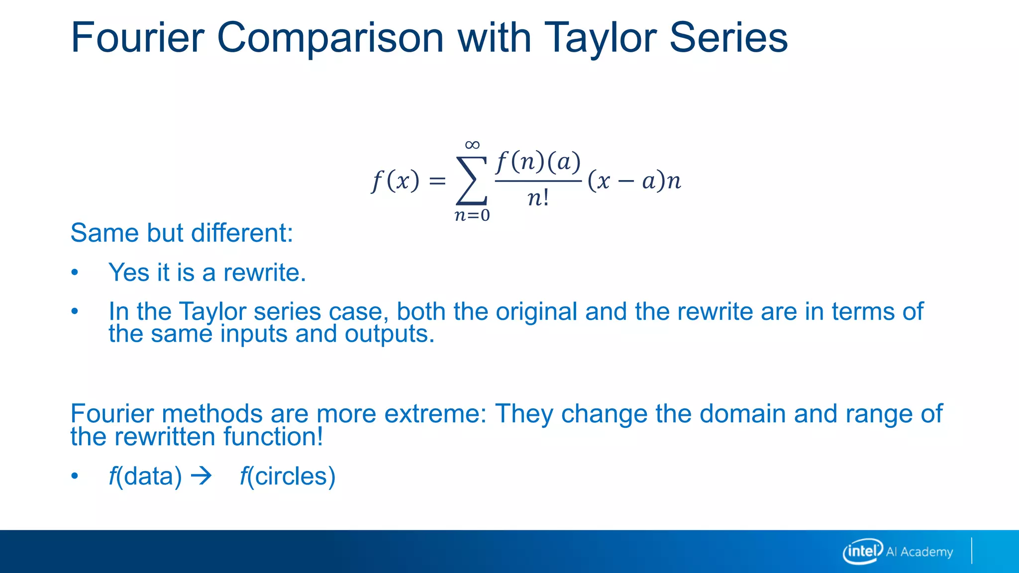
Fourier Comparison with Taylor Series
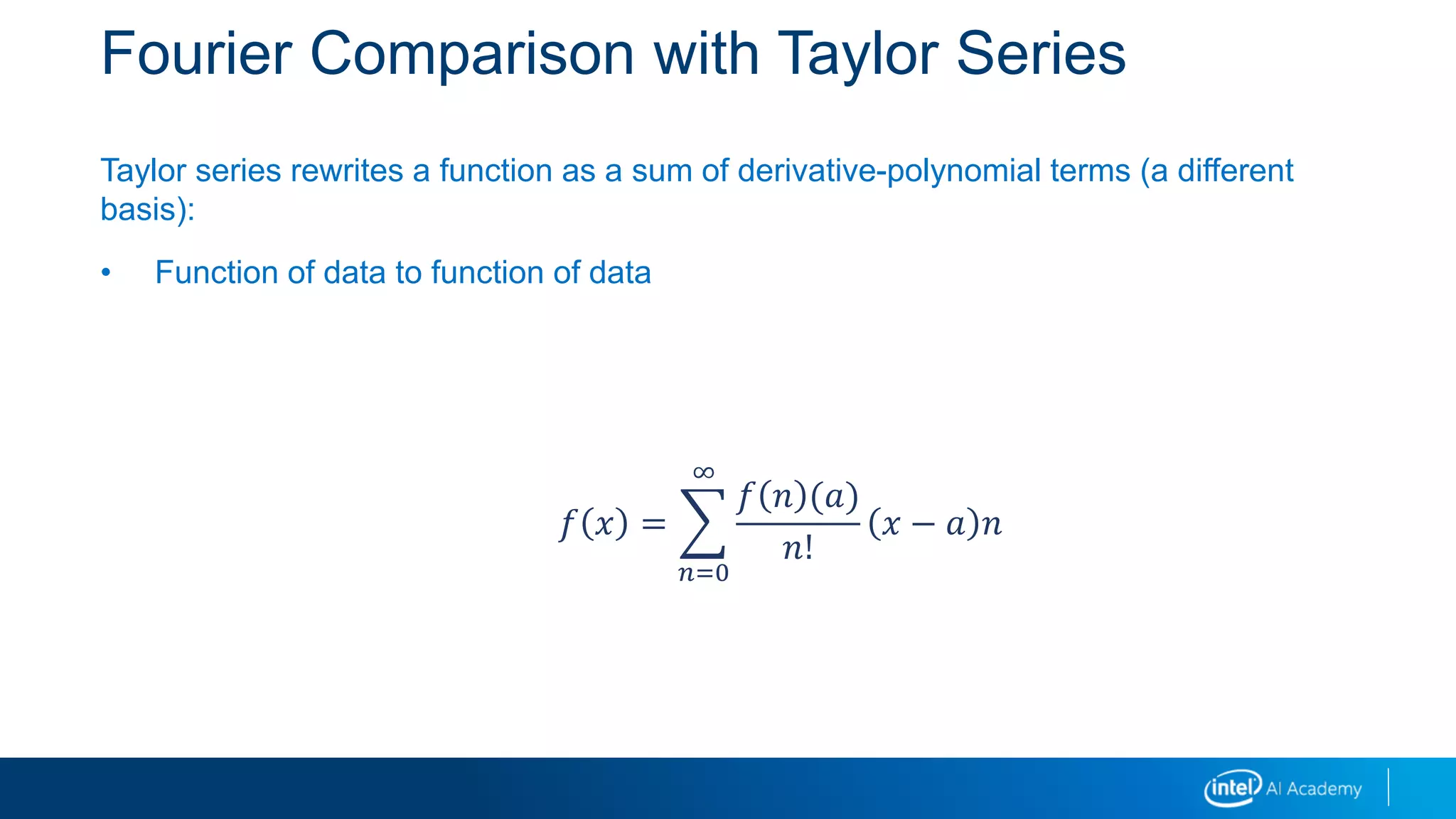
Taylor series rewrites a function as a sum of derivative-polynomial terms (a different
basis):
β€’ Function of data to function of data
𝑓 π‘₯ =
𝑛=0
∞
𝑓 𝑛 (π‘Ž)
𝑛!
π‘₯ βˆ’ π‘Ž 𝑛
Fourier Comparison with Taylor Series
Same but different:
β€’ Yes it is a rewrite.
β€’ In the Taylor series case, both the original and the rewrite are in terms of
the same inputs and outputs.
Fourier methods are more extreme: They change the domain and range of
the rewritten function!
β€’ f(data) οƒ  f(circles)
𝑓 π‘₯ =
𝑛=0
∞
𝑓 𝑛 (π‘Ž)
𝑛!
π‘₯ βˆ’ π‘Ž 𝑛
FFT and DFT
We will be using one pair of Fourier methods.
Forward: Data to circle
Backward: Circle to data
FFT and DFT: Forward
Forward: Data to circle
Input fdata([0,N-1]]) οƒ 
Output fcircles([0,N-1])
The input function tells us our data values
Input has N data values
Output has N circles
The output function tells us characteristics of the circles in our rewrites
FFT and DFT: Backward
Backward: Circle to data
Input fcircles([0,N-1]]) οƒ 
Output fdata([0,N-1])
Here we are going from an input function in terms of circles to an output
function in terms of our data
Input has N circles
Output has N data values
FFT and DFT: p
You might be worried that neither of these are necessarily functions of, or around, a
circle.
What is a function of a circle?
β€’ A function of a circle is defined for each angle of a walk around a circle [0, 2p]
radians
FFT and DFT: p
We can convert to a function of a circle if
1. Our input is discrete and finite:
Map our values from [0, N-1] to points around the circle
Divide [0, 2p] into N parts
This is what we have with images
 Images are discrete and finite
 Edges of the images wrap to make a circle
2. Our input is discrete and repeating:
Do the exact same thing because the circle wraps around itself!
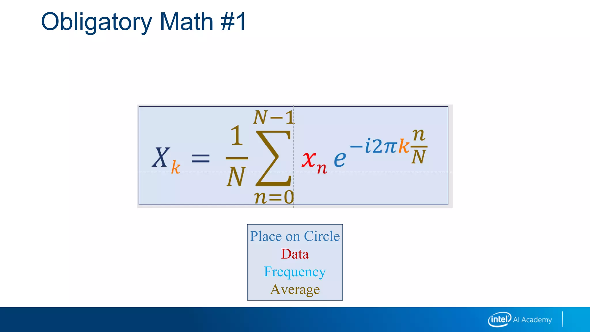
Obligatory Math #1
π‘‹π‘˜ =
1
𝑁
𝑛=0
π‘βˆ’1
π‘₯𝑛 π‘’βˆ’π‘–2πœ‹π‘˜
𝑛
𝑁
Place on Circle
Data
Frequency
Average
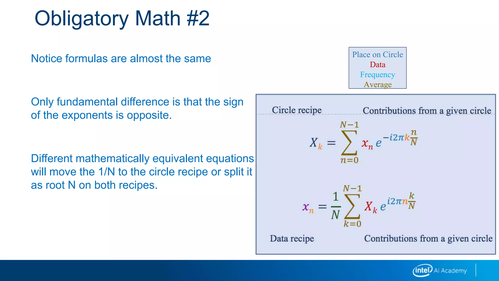
Obligatory Math #2
Notice formulas are almost the same
Only fundamental difference is that the sign
of the exponents is opposite.
Different mathematically equivalent equations
will move the 1/N to the circle recipe or split it
as root N on both recipes.
Circle recipe Contributions from a given circle
π‘‹π‘˜ =
𝑛=0
π‘βˆ’1
π‘₯𝑛 π‘’βˆ’π‘–2πœ‹π‘˜
𝑛
𝑁
Data recipe Contributions from a given circle
π‘₯𝑛 =
1
𝑁
π‘˜=0
π‘βˆ’1
π‘‹π‘˜ 𝑒 𝑖2πœ‹π‘›
π‘˜
𝑁
Place on Circle
Data
Frequency
Average
Why Fourier?
Filtering
Fast convolutions
Compression
β€’ See JPEG and MP3s!
Why Fourier?
Our rewrite in terms of circles can be hacked.
Different circles move at different speeds
β€’ For example, we even have a term for the stationary circle: the mean
Speeds (frequencies) are related to image regions of slow and fast variation
β€’ High-speed changes are either edges or noise
Low-speed changes are, taken together, a peculiar averaging of the data.
Why Fourier?
These give us:
High-pass filters where we keep high frequencies.
Low-pass filters where we keep low frequencies.
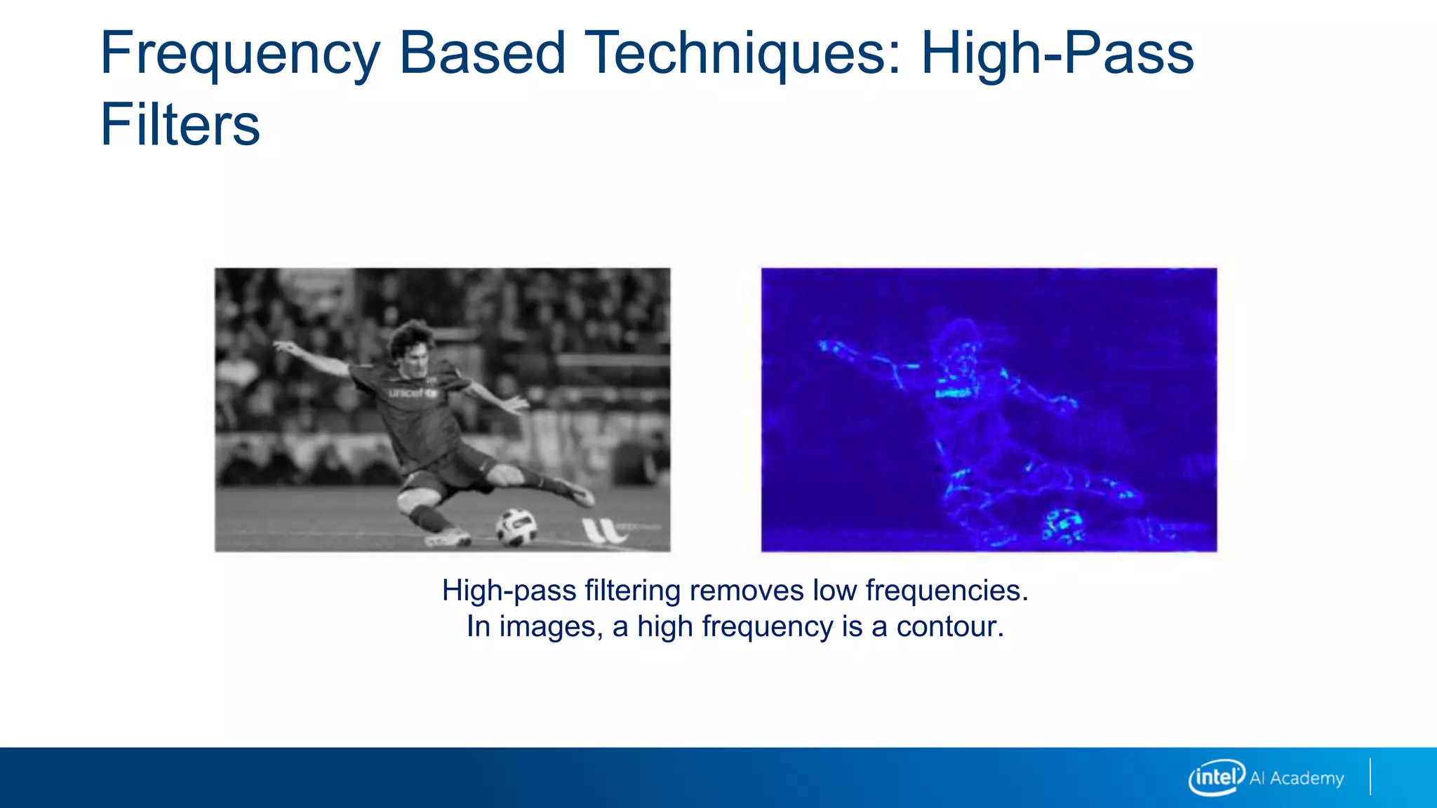
Frequency Based Techniques: High-Pass
Filters
High-pass filtering removes low frequencies.
In images, a high frequency is a contour.
Why Fourier?
We can take advantage of properties of Fourier transforms.
Convolutions, in circle space, are simply multiplication.
This can allow us to drastically speed up convolutions:
1. Discrete Fourier transform (DFT) the data and the kernel
2. Perform multiplication in circle space
3. Transform back to data space
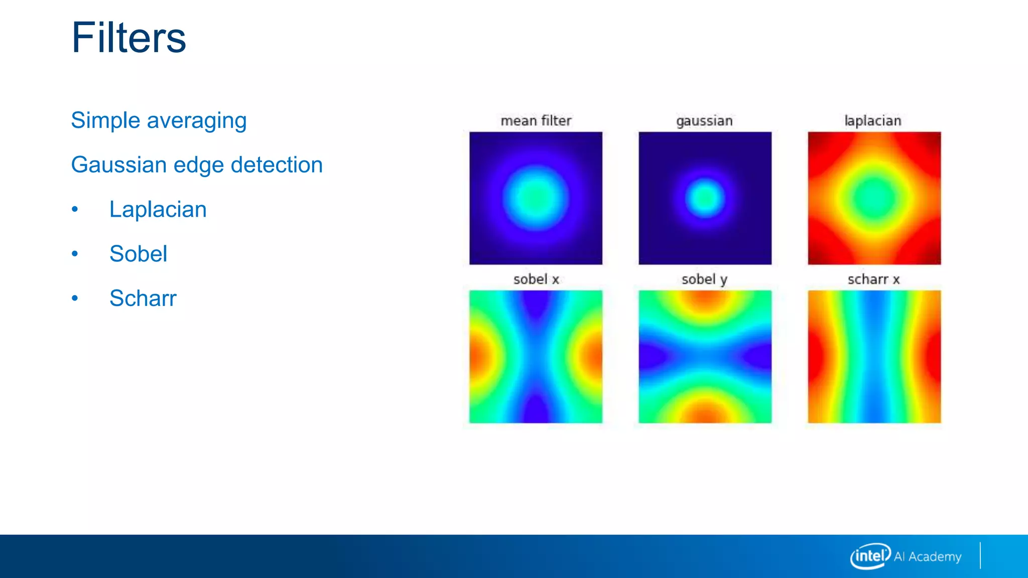
Filters
Simple averaging
Gaussian edge detection
β€’ Laplacian
β€’ Sobel
β€’ Scharr
How to Use Fourier Methods
NumPy and OpenCV (and others):
β€’ It uses the fast Fourier transform to compute the discrete Fourier transform.
Gives data points from an underlying, unknown function
β€’ There are usually some variations for dealing with different types of input.
β€’ There are variations for whether we are going forward (to circle space) or
backwards (to data space).
How to Use Fourier Methods
There are usually some helper functions to deal with the weirdness of
implementation details.
One important detail is that of size:
 DFT algorithms are designed to work best with particular sizes
 Different implementations subdivide the problem into different sizes, so
they have different ideal input sizes
– NumPy implementation ideal size is a power of 2
– OpenCV implementation ideal size is a product of 2s, 3s, 5s
– For example, 2*2*3*5*5 = 300
For OpenCV, we can calculate with cv2.getOptimalDFTSize().
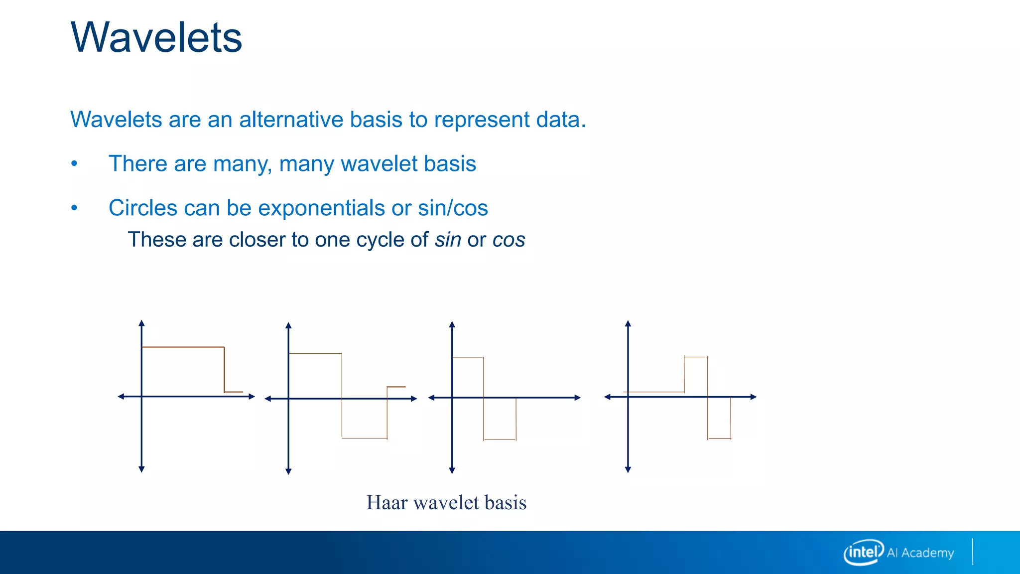
Wavelets
Wavelets are an alternative basis to represent data.
β€’ There are many, many wavelet basis
β€’ Circles can be exponentials or sin/cos
These are closer to one cycle of sin or cos
Haar wavelet basis
Wavelets
A data representation describes the phenomena point-by-point.
Circle space describes the data in terms of cycles.
Wavelets represent a tradeoff between the two.
Wavelets
We can tell something about both the data and the circle characteristics at the same
time.
But …
β€’ We can’t know both exactly.
β€’ Amazingly, this is the mathematical root of one version of the Heisenberg
Uncertainty Principle.
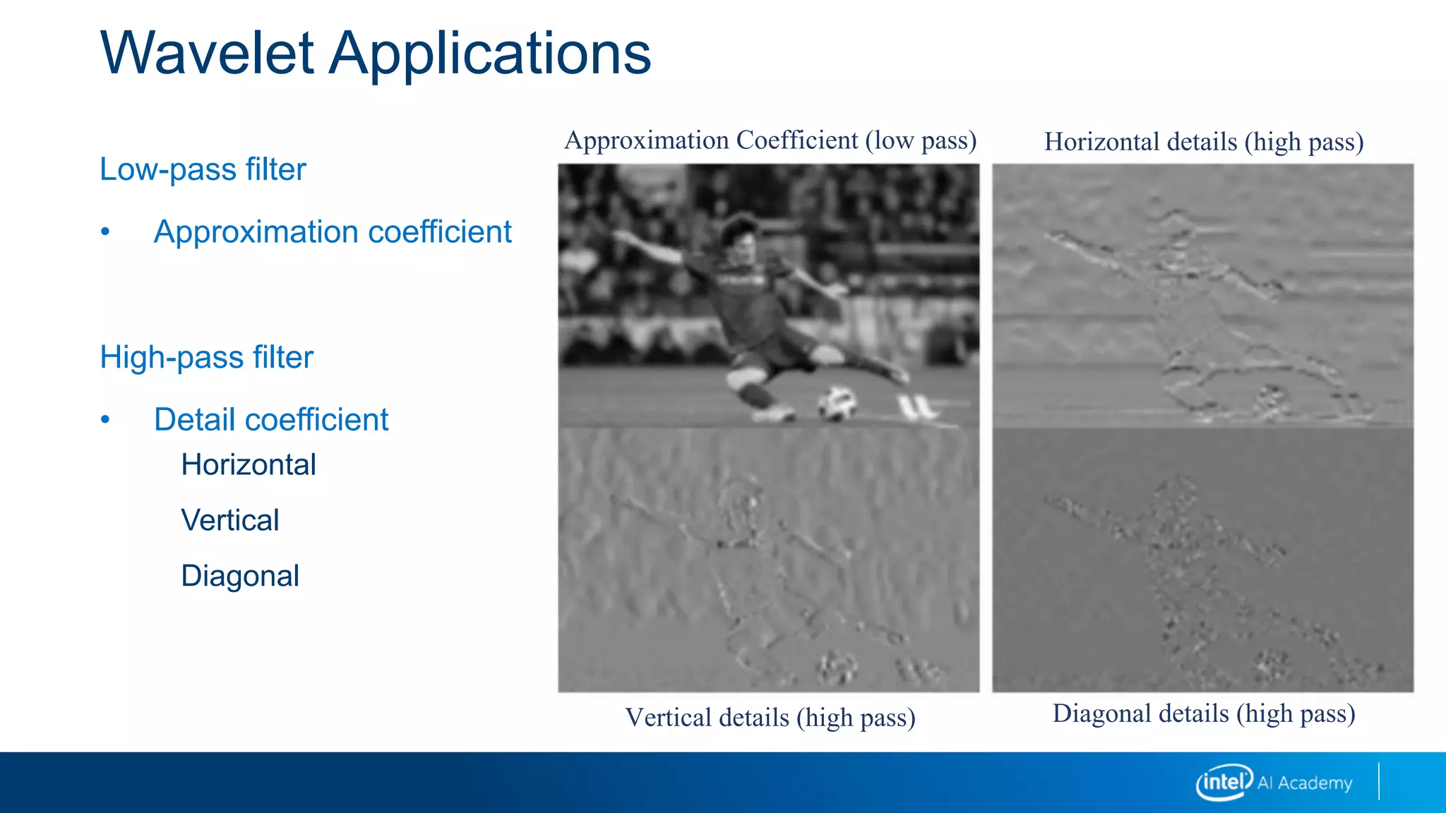
Wavelet Applications
Wavelets are:
β€’ Used for denoising
β€’ Used for compression
β€’ May outperform DFT and discrete cosine transform (DCT) in peak detection
Wavelet Applications
Low-pass filter
β€’ Approximation coefficient
High-pass filter
β€’ Detail coefficient
Horizontal
Vertical
Diagonal
Approximation Coefficient (low pass) Horizontal details (high pass)
Vertical details (high pass) Diagonal details (high pass)
Discrete Wavelet Transform
Similar to the FFT and DFT, we use the discrete wavelet transform (DWT).
We use the PyWavelets* (pywt) package to do the calculations.
import pywt
cA2, (cH2, cV2, cD2), (cH1, cV1, cD1) =
pywt.wavedec2(messi, 'haar', level=2)
Discrete Wavelet Transform
Level is similar to levels in a Gaussian pyramid:
β€’ One application of DWT results in an approximate image and details.
We can add the two to get back the original image
β€’ Subsequent applications of DWT on the level 1 approximate image give us a level 2
approximate image and level 2 detail images.
β€’ We can continue applying this process recursively.
Line Detection: Successive Approximation
Transforming from a curve-contour to a simpler representation (aka line simplification)
Piecewise-linear polyline
B-spline curve
If the contour is a line (with noise) we can simplify it to that line.
If not, the line simplification is used to approximate the original curve.
Hough Transforms
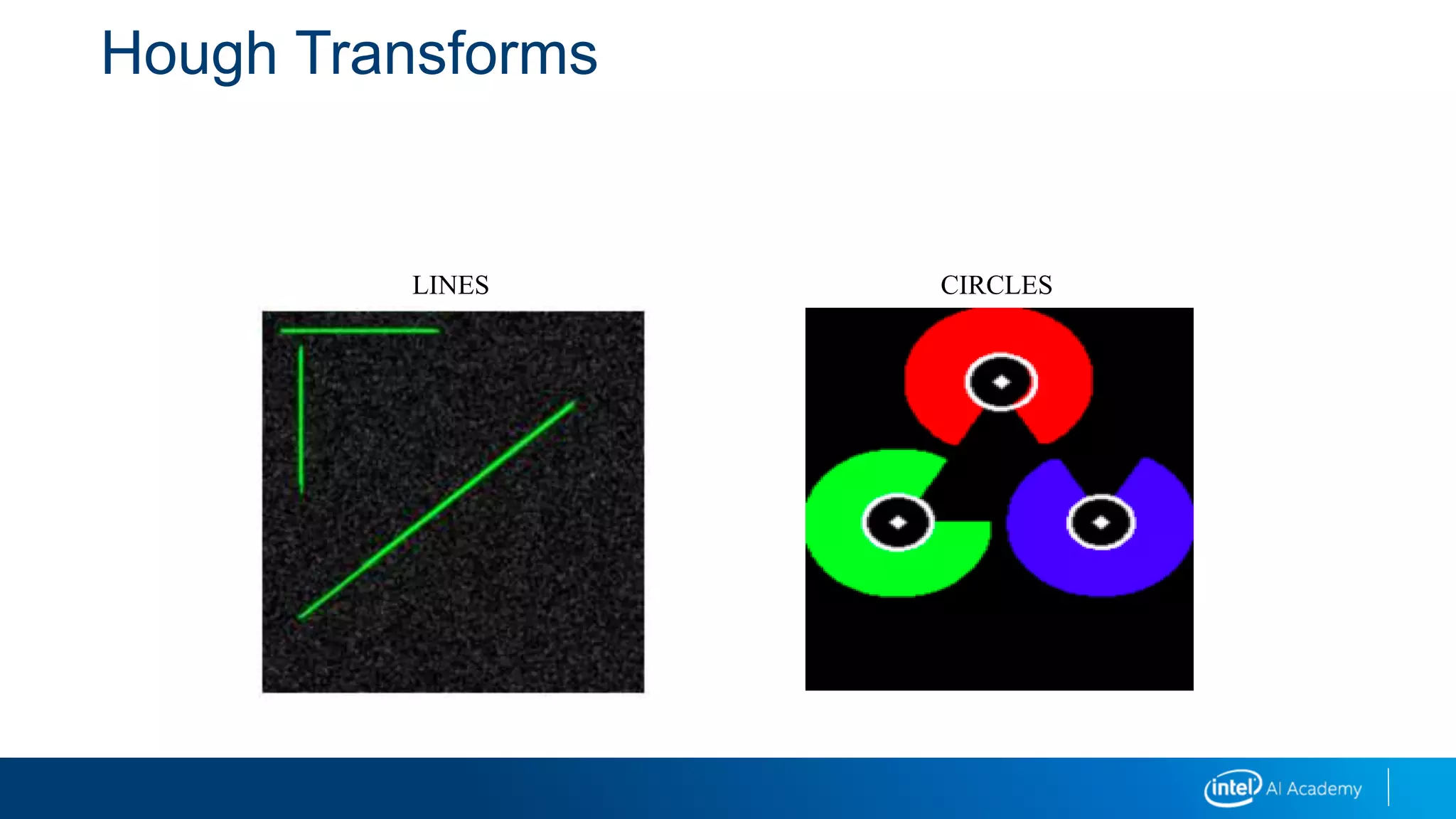
Propose shape from point
Count points that agree with shape
Keep shapes at points with highest counts
Can do this for any shape we can describe with a small number of parameters (such as
point-slope, angle-distance, center-radius, center-scale-angle).
Hough Transforms
LINES CIRCLES
Hough Transforms: An Example
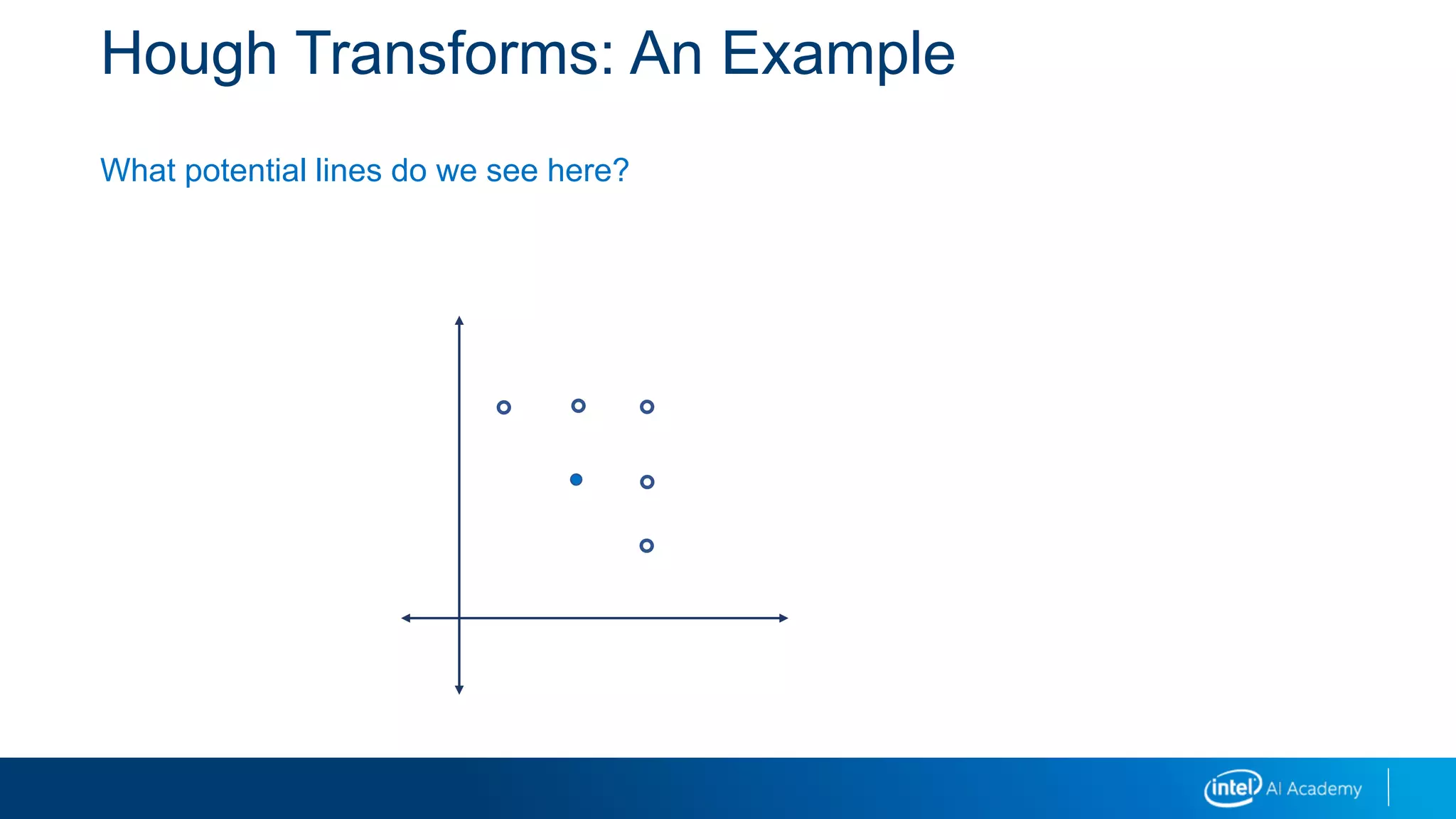
What potential lines do we see here?
Hough Transforms: An Example
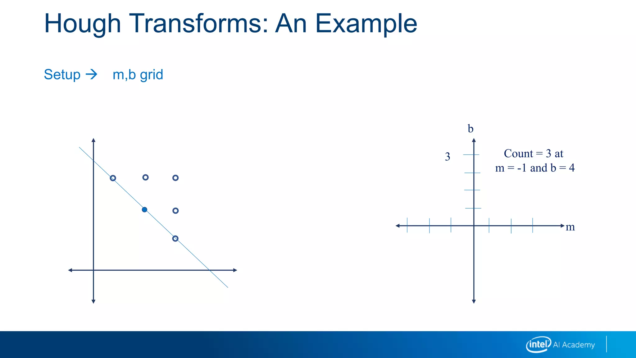
Setup οƒ  m,b grid
Count = 3 at
m = -1 and b = 4
m
b
3
Hough Transforms: An Example
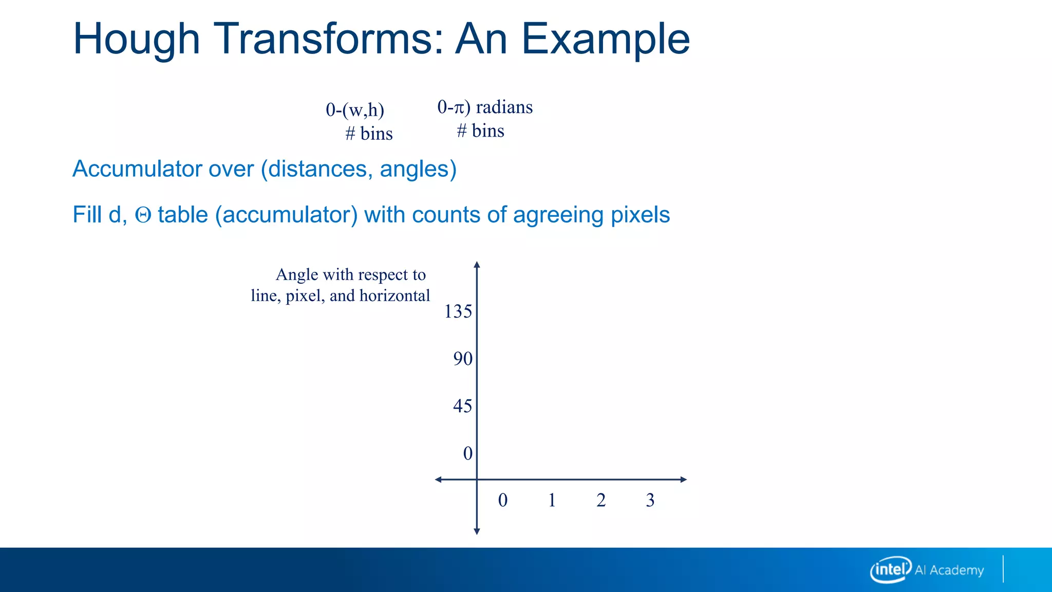
Accumulator over (distances, angles)
Fill d, Q table (accumulator) with counts of agreeing pixels
0-(w,h)
# bins
0-p) radians
# bins
0 1 2 3
135
90
45
0
Angle with respect to
line, pixel, and horizontal
Hough Transforms: An Example
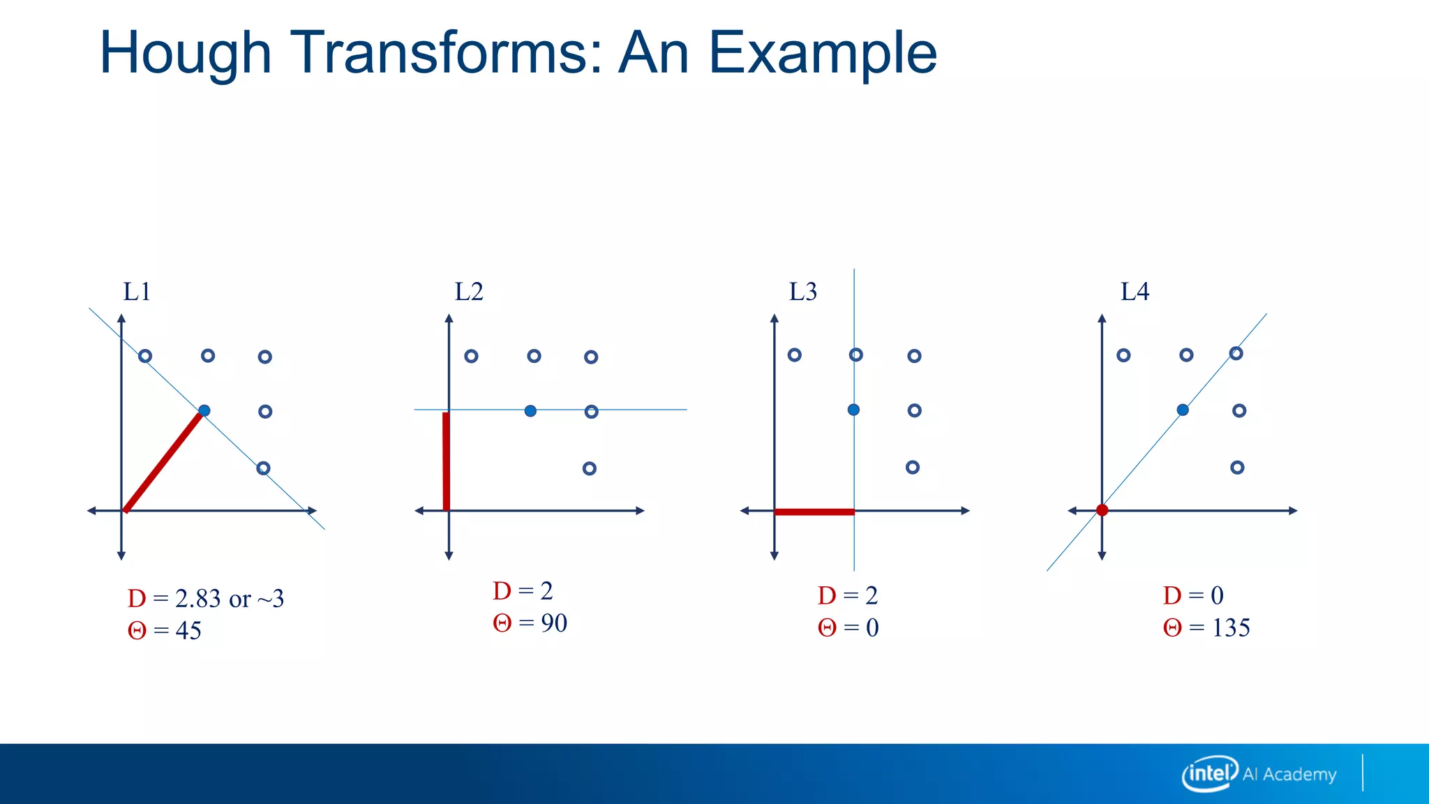
L1 L2 L3 L4
D = 2.83 or ~3
Q = 45
D = 2
Q = 90
D = 2
Q = 0
D = 0
Q = 135
Hough Transforms: An Example
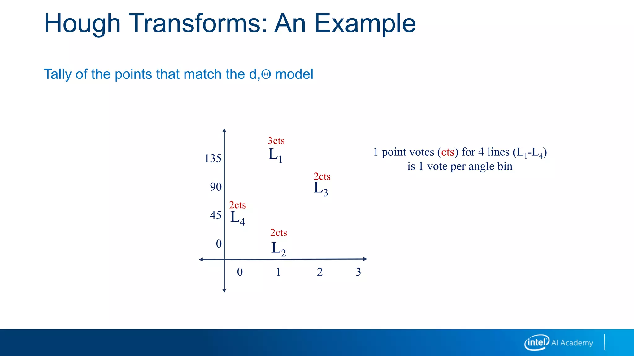
Tally of the points that match the d,Q model
0 1 2 3
135
90
45
0
L1
L2
L4
L3
2cts
3cts
2cts
2cts
1 point votes (cts) for 4 lines (L1-L4)
is 1 vote per angle bin
Hough Circle Transform
The circle is similar to the lines
But, the vote is performed by taking the circle center and its radius
Three parameters in this case
Would be too slow because of combinatorics
Would produce a very sparse table because of relatively few matching objects
Instead, we use the gradient and combined edges
Only the connected can vote for the same circle
General Hough Transform
We can generalize this process to other shapes by using a contour instead of the
perimeter of the circle.
Track from a pixel on the contour, rotate the orientation of the contour around a circle
β€’ Count pixels matching at angles.
β€’ Can also have scaling factors.
Line Detection: RANdom SAmple Consensus
(RANSAC)Pair of edge elements are used to form a line hypothesis.
How many others fall on this line?
Set boundaries for minimum matchers
Can also use RANSAC for image alignment.
Note: see OpenCV fitLine:
It may use a RANSAC-like method
Is it RANSAC-like only in use of m-estimator?
Edge Thinning: Detecting Thick Edges
Detect thick edges as one edge (without doubling)
Morphological erosion
Skeletonization
Watershed
Pearling
Convert edges to contours
 findCountours()
Line Detection: Hough Transforms
For occluded lines, we need more advanced techniques like Hough transform.
β€’ NOTE: Hough can include or exclude gradient information.
β€’ With it:
Do not need to orient the line
Need fewer accumulators
Do not need inner loop (work has already been done)

More Related Content

What's hot

Machine learning and_nlp
Machine learning and_nlpMachine learning and_nlp
Machine learning and_nlpankit_ppt
Β 
Convolutional Neural Network (CNN) presentation from theory to code in Theano
Convolutional Neural Network (CNN) presentation from theory to code in TheanoConvolutional Neural Network (CNN) presentation from theory to code in Theano
Convolutional Neural Network (CNN) presentation from theory to code in TheanoSeongwon Hwang
Β 
Machine Learning - Introduction to Convolutional Neural Networks
Machine Learning - Introduction to Convolutional Neural NetworksMachine Learning - Introduction to Convolutional Neural Networks
Machine Learning - Introduction to Convolutional Neural NetworksAndrew Ferlitsch
Β 
Deep learning summary
Deep learning summaryDeep learning summary
Deep learning summaryankit_ppt
Β 
Image processing
Image processingImage processing
Image processingmaheshpene
Β 
Foundations: Artificial Neural Networks
Foundations: Artificial Neural NetworksFoundations: Artificial Neural Networks
Foundations: Artificial Neural Networksananth
Β 
Deep learning: Mathematical Perspective
Deep learning: Mathematical PerspectiveDeep learning: Mathematical Perspective
Deep learning: Mathematical PerspectiveYounusS2
Β 
Kohonen self organizing maps
Kohonen self organizing mapsKohonen self organizing maps
Kohonen self organizing mapsraphaelkiminya
Β 
Support Vector Machines
Support Vector MachinesSupport Vector Machines
Support Vector Machinesnextlib
Β 
Basics of Machine Learning
Basics of Machine LearningBasics of Machine Learning
Basics of Machine LearningPranav Challa
Β 
Hands-On Machine Learning with Scikit-Learn and TensorFlow - Chapter8
Hands-On Machine Learning with Scikit-Learn and TensorFlow - Chapter8Hands-On Machine Learning with Scikit-Learn and TensorFlow - Chapter8
Hands-On Machine Learning with Scikit-Learn and TensorFlow - Chapter8Hakky St
Β 
Data Science - Part IX - Support Vector Machine
Data Science - Part IX -  Support Vector MachineData Science - Part IX -  Support Vector Machine
Data Science - Part IX - Support Vector MachineDerek Kane
Β 
Deep Feed Forward Neural Networks and Regularization
Deep Feed Forward Neural Networks and RegularizationDeep Feed Forward Neural Networks and Regularization
Deep Feed Forward Neural Networks and RegularizationYan Xu
Β 
Histogram Processing
Histogram ProcessingHistogram Processing
Histogram ProcessingAmnaakhaan
Β 
Introduction to Image Processing with MATLAB
Introduction to Image Processing with MATLABIntroduction to Image Processing with MATLAB
Introduction to Image Processing with MATLABSriram Emarose
Β 
Variational Autoencoders For Image Generation
Variational Autoencoders For Image GenerationVariational Autoencoders For Image Generation
Variational Autoencoders For Image GenerationJason Anderson
Β 

What's hot (20)

Machine learning and_nlp
Machine learning and_nlpMachine learning and_nlp
Machine learning and_nlp
Β 
Convolutional Neural Network (CNN) presentation from theory to code in Theano
Convolutional Neural Network (CNN) presentation from theory to code in TheanoConvolutional Neural Network (CNN) presentation from theory to code in Theano
Convolutional Neural Network (CNN) presentation from theory to code in Theano
Β 
Machine Learning - Introduction to Convolutional Neural Networks
Machine Learning - Introduction to Convolutional Neural NetworksMachine Learning - Introduction to Convolutional Neural Networks
Machine Learning - Introduction to Convolutional Neural Networks
Β 
Deep learning summary
Deep learning summaryDeep learning summary
Deep learning summary
Β 
Image processing
Image processingImage processing
Image processing
Β 
Foundations: Artificial Neural Networks
Foundations: Artificial Neural NetworksFoundations: Artificial Neural Networks
Foundations: Artificial Neural Networks
Β 
Deep learning: Mathematical Perspective
Deep learning: Mathematical PerspectiveDeep learning: Mathematical Perspective
Deep learning: Mathematical Perspective
Β 
Kohonen self organizing maps
Kohonen self organizing mapsKohonen self organizing maps
Kohonen self organizing maps
Β 
Lesson 39
Lesson 39Lesson 39
Lesson 39
Β 
Support Vector Machines
Support Vector MachinesSupport Vector Machines
Support Vector Machines
Β 
Basics of Machine Learning
Basics of Machine LearningBasics of Machine Learning
Basics of Machine Learning
Β 
Lesson 38
Lesson 38Lesson 38
Lesson 38
Β 
Hands-On Machine Learning with Scikit-Learn and TensorFlow - Chapter8
Hands-On Machine Learning with Scikit-Learn and TensorFlow - Chapter8Hands-On Machine Learning with Scikit-Learn and TensorFlow - Chapter8
Hands-On Machine Learning with Scikit-Learn and TensorFlow - Chapter8
Β 
Data Science - Part IX - Support Vector Machine
Data Science - Part IX -  Support Vector MachineData Science - Part IX -  Support Vector Machine
Data Science - Part IX - Support Vector Machine
Β 
Deep Feed Forward Neural Networks and Regularization
Deep Feed Forward Neural Networks and RegularizationDeep Feed Forward Neural Networks and Regularization
Deep Feed Forward Neural Networks and Regularization
Β 
Lesson 36
Lesson 36Lesson 36
Lesson 36
Β 
PCA and SVD in brief
PCA and SVD in briefPCA and SVD in brief
PCA and SVD in brief
Β 
Histogram Processing
Histogram ProcessingHistogram Processing
Histogram Processing
Β 
Introduction to Image Processing with MATLAB
Introduction to Image Processing with MATLABIntroduction to Image Processing with MATLAB
Introduction to Image Processing with MATLAB
Β 
Variational Autoencoders For Image Generation
Variational Autoencoders For Image GenerationVariational Autoencoders For Image Generation
Variational Autoencoders For Image Generation
Β 

Similar to 04 image transformations_ii

Lecture 9-online
Lecture 9-onlineLecture 9-online
Lecture 9-onlinelifebreath
Β 
Basics of edge detection and forier transform
Basics of edge detection and forier transformBasics of edge detection and forier transform
Basics of edge detection and forier transformSimranjit Singh
Β 
Robust and Tuneable Family of Gossiping Algorithms
Robust and Tuneable Family of Gossiping AlgorithmsRobust and Tuneable Family of Gossiping Algorithms
Robust and Tuneable Family of Gossiping AlgorithmsVincenzo De Florio
Β 
CS6640_F2014_Fourier_I.pdf
CS6640_F2014_Fourier_I.pdfCS6640_F2014_Fourier_I.pdf
CS6640_F2014_Fourier_I.pdfSsdSsd5
Β 
Wavelet Based Image Compression Using FPGA
Wavelet Based Image Compression Using FPGAWavelet Based Image Compression Using FPGA
Wavelet Based Image Compression Using FPGADr. Mohieddin Moradi
Β 
Lec 07 image enhancement in frequency domain i
Lec 07 image enhancement in frequency domain iLec 07 image enhancement in frequency domain i
Lec 07 image enhancement in frequency domain iAli Hassan
Β 
Introduction to Digital Signal Processing (DSP) - Course Notes
Introduction to Digital Signal Processing (DSP) - Course NotesIntroduction to Digital Signal Processing (DSP) - Course Notes
Introduction to Digital Signal Processing (DSP) - Course NotesAhmed Gad
Β 
APPLIED MACHINE LEARNING
APPLIED MACHINE LEARNINGAPPLIED MACHINE LEARNING
APPLIED MACHINE LEARNINGRevanth Kumar
Β 
Daubechies wavelets
Daubechies waveletsDaubechies wavelets
Daubechies waveletsDANISHAMIN950
Β 
Loop parallelization & pipelining
Loop parallelization & pipeliningLoop parallelization & pipelining
Loop parallelization & pipeliningjagrat123
Β 
affine transformation for computer graphics
affine transformation for computer graphicsaffine transformation for computer graphics
affine transformation for computer graphicsDrSUGANYADEVIK
Β 
Frequency Response with MATLAB Examples.pdf
Frequency Response with MATLAB Examples.pdfFrequency Response with MATLAB Examples.pdf
Frequency Response with MATLAB Examples.pdfSunil Manjani
Β 
Fft analysis
Fft analysisFft analysis
Fft analysisSatrious
Β 

Similar to 04 image transformations_ii (20)

ME-314- Control Engineering - Week 02
ME-314- Control Engineering - Week 02ME-314- Control Engineering - Week 02
ME-314- Control Engineering - Week 02
Β 
Lecture 9-online
Lecture 9-onlineLecture 9-online
Lecture 9-online
Β 
Basics of edge detection and forier transform
Basics of edge detection and forier transformBasics of edge detection and forier transform
Basics of edge detection and forier transform
Β 
Robust and Tuneable Family of Gossiping Algorithms
Robust and Tuneable Family of Gossiping AlgorithmsRobust and Tuneable Family of Gossiping Algorithms
Robust and Tuneable Family of Gossiping Algorithms
Β 
CS6640_F2014_Fourier_I.pdf
CS6640_F2014_Fourier_I.pdfCS6640_F2014_Fourier_I.pdf
CS6640_F2014_Fourier_I.pdf
Β 
Wavelet Based Image Compression Using FPGA
Wavelet Based Image Compression Using FPGAWavelet Based Image Compression Using FPGA
Wavelet Based Image Compression Using FPGA
Β 
CO3303-2 Lecture.ppt
CO3303-2 Lecture.pptCO3303-2 Lecture.ppt
CO3303-2 Lecture.ppt
Β 
PS
PSPS
PS
Β 
Lec 07 image enhancement in frequency domain i
Lec 07 image enhancement in frequency domain iLec 07 image enhancement in frequency domain i
Lec 07 image enhancement in frequency domain i
Β 
DeepLearning.pdf
DeepLearning.pdfDeepLearning.pdf
DeepLearning.pdf
Β 
Introduction to Digital Signal Processing (DSP) - Course Notes
Introduction to Digital Signal Processing (DSP) - Course NotesIntroduction to Digital Signal Processing (DSP) - Course Notes
Introduction to Digital Signal Processing (DSP) - Course Notes
Β 
APPLIED MACHINE LEARNING
APPLIED MACHINE LEARNINGAPPLIED MACHINE LEARNING
APPLIED MACHINE LEARNING
Β 
Daubechies wavelets
Daubechies waveletsDaubechies wavelets
Daubechies wavelets
Β 
Lec11.ppt
Lec11.pptLec11.ppt
Lec11.ppt
Β 
Loop parallelization & pipelining
Loop parallelization & pipeliningLoop parallelization & pipelining
Loop parallelization & pipelining
Β 
affine transformation for computer graphics
affine transformation for computer graphicsaffine transformation for computer graphics
affine transformation for computer graphics
Β 
Frequency Response with MATLAB Examples.pdf
Frequency Response with MATLAB Examples.pdfFrequency Response with MATLAB Examples.pdf
Frequency Response with MATLAB Examples.pdf
Β 
F0153236
F0153236F0153236
F0153236
Β 
FFT Analysis
FFT AnalysisFFT Analysis
FFT Analysis
Β 
Fft analysis
Fft analysisFft analysis
Fft analysis
Β 

More from ankit_ppt

01 foundations
01 foundations01 foundations
01 foundationsankit_ppt
Β 
Word2 vec
Word2 vecWord2 vec
Word2 vecankit_ppt
Β 
Text similarity measures
Text similarity measuresText similarity measures
Text similarity measuresankit_ppt
Β 
Text generation and_advanced_topics
Text generation and_advanced_topicsText generation and_advanced_topics
Text generation and_advanced_topicsankit_ppt
Β 
Nlp toolkits and_preprocessing_techniques
Nlp toolkits and_preprocessing_techniquesNlp toolkits and_preprocessing_techniques
Nlp toolkits and_preprocessing_techniquesankit_ppt
Β 
Latent dirichlet allocation_and_topic_modeling
Latent dirichlet allocation_and_topic_modelingLatent dirichlet allocation_and_topic_modeling
Latent dirichlet allocation_and_topic_modelingankit_ppt
Β 
Intro to nlp
Intro to nlpIntro to nlp
Intro to nlpankit_ppt
Β 
Ot regularization and_gradient_descent
Ot regularization and_gradient_descentOt regularization and_gradient_descent
Ot regularization and_gradient_descentankit_ppt
Β 
Ml9 introduction to-unsupervised_learning_and_clustering_methods
Ml9 introduction to-unsupervised_learning_and_clustering_methodsMl9 introduction to-unsupervised_learning_and_clustering_methods
Ml9 introduction to-unsupervised_learning_and_clustering_methodsankit_ppt
Β 
Ml8 boosting and-stacking
Ml8 boosting and-stackingMl8 boosting and-stacking
Ml8 boosting and-stackingankit_ppt
Β 
Ml7 bagging
Ml7 baggingMl7 bagging
Ml7 baggingankit_ppt
Β 
Ml6 decision trees
Ml6 decision treesMl6 decision trees
Ml6 decision treesankit_ppt
Β 
Ml5 svm and-kernels
Ml5 svm and-kernelsMl5 svm and-kernels
Ml5 svm and-kernelsankit_ppt
Β 
Ml4 naive bayes
Ml4 naive bayesMl4 naive bayes
Ml4 naive bayesankit_ppt
Β 
Lesson 3 ai in the enterprise
Lesson 3   ai in the enterpriseLesson 3   ai in the enterprise
Lesson 3 ai in the enterpriseankit_ppt
Β 
Ml3 logistic regression-and_classification_error_metrics
Ml3 logistic regression-and_classification_error_metricsMl3 logistic regression-and_classification_error_metrics
Ml3 logistic regression-and_classification_error_metricsankit_ppt
Β 
Ml2 train test-splits_validation_linear_regression
Ml2 train test-splits_validation_linear_regressionMl2 train test-splits_validation_linear_regression
Ml2 train test-splits_validation_linear_regressionankit_ppt
Β 
Ml1 introduction to-supervised_learning_and_k_nearest_neighbors
Ml1 introduction to-supervised_learning_and_k_nearest_neighborsMl1 introduction to-supervised_learning_and_k_nearest_neighbors
Ml1 introduction to-supervised_learning_and_k_nearest_neighborsankit_ppt
Β 
Lesson 2 ai in industry
Lesson 2   ai in industryLesson 2   ai in industry
Lesson 2 ai in industryankit_ppt
Β 
Lesson 5 arima
Lesson 5 arimaLesson 5 arima
Lesson 5 arimaankit_ppt
Β 

More from ankit_ppt (20)

01 foundations
01 foundations01 foundations
01 foundations
Β 
Word2 vec
Word2 vecWord2 vec
Word2 vec
Β 
Text similarity measures
Text similarity measuresText similarity measures
Text similarity measures
Β 
Text generation and_advanced_topics
Text generation and_advanced_topicsText generation and_advanced_topics
Text generation and_advanced_topics
Β 
Nlp toolkits and_preprocessing_techniques
Nlp toolkits and_preprocessing_techniquesNlp toolkits and_preprocessing_techniques
Nlp toolkits and_preprocessing_techniques
Β 
Latent dirichlet allocation_and_topic_modeling
Latent dirichlet allocation_and_topic_modelingLatent dirichlet allocation_and_topic_modeling
Latent dirichlet allocation_and_topic_modeling
Β 
Intro to nlp
Intro to nlpIntro to nlp
Intro to nlp
Β 
Ot regularization and_gradient_descent
Ot regularization and_gradient_descentOt regularization and_gradient_descent
Ot regularization and_gradient_descent
Β 
Ml9 introduction to-unsupervised_learning_and_clustering_methods
Ml9 introduction to-unsupervised_learning_and_clustering_methodsMl9 introduction to-unsupervised_learning_and_clustering_methods
Ml9 introduction to-unsupervised_learning_and_clustering_methods
Β 
Ml8 boosting and-stacking
Ml8 boosting and-stackingMl8 boosting and-stacking
Ml8 boosting and-stacking
Β 
Ml7 bagging
Ml7 baggingMl7 bagging
Ml7 bagging
Β 
Ml6 decision trees
Ml6 decision treesMl6 decision trees
Ml6 decision trees
Β 
Ml5 svm and-kernels
Ml5 svm and-kernelsMl5 svm and-kernels
Ml5 svm and-kernels
Β 
Ml4 naive bayes
Ml4 naive bayesMl4 naive bayes
Ml4 naive bayes
Β 
Lesson 3 ai in the enterprise
Lesson 3   ai in the enterpriseLesson 3   ai in the enterprise
Lesson 3 ai in the enterprise
Β 
Ml3 logistic regression-and_classification_error_metrics
Ml3 logistic regression-and_classification_error_metricsMl3 logistic regression-and_classification_error_metrics
Ml3 logistic regression-and_classification_error_metrics
Β 
Ml2 train test-splits_validation_linear_regression
Ml2 train test-splits_validation_linear_regressionMl2 train test-splits_validation_linear_regression
Ml2 train test-splits_validation_linear_regression
Β 
Ml1 introduction to-supervised_learning_and_k_nearest_neighbors
Ml1 introduction to-supervised_learning_and_k_nearest_neighborsMl1 introduction to-supervised_learning_and_k_nearest_neighbors
Ml1 introduction to-supervised_learning_and_k_nearest_neighbors
Β 
Lesson 2 ai in industry
Lesson 2   ai in industryLesson 2   ai in industry
Lesson 2 ai in industry
Β 
Lesson 5 arima
Lesson 5 arimaLesson 5 arima
Lesson 5 arima
Β 

Recently uploaded

DJARUM4D - SLOT GACOR ONLINE | SLOT DEMO ONLINE
DJARUM4D - SLOT GACOR ONLINE | SLOT DEMO ONLINEDJARUM4D - SLOT GACOR ONLINE | SLOT DEMO ONLINE
DJARUM4D - SLOT GACOR ONLINE | SLOT DEMO ONLINEslot gacor bisa pakai pulsa
Β 
The Most Attractive Pune Call Girls Budhwar Peth 8250192130 Will You Miss Thi...
The Most Attractive Pune Call Girls Budhwar Peth 8250192130 Will You Miss Thi...The Most Attractive Pune Call Girls Budhwar Peth 8250192130 Will You Miss Thi...
The Most Attractive Pune Call Girls Budhwar Peth 8250192130 Will You Miss Thi...ranjana rawat
Β 
SPICE PARK APR2024 ( 6,793 SPICE Models )
SPICE PARK APR2024 ( 6,793 SPICE Models )SPICE PARK APR2024 ( 6,793 SPICE Models )
SPICE PARK APR2024 ( 6,793 SPICE Models )Tsuyoshi Horigome
Β 
(PRIYA) Rajgurunagar Call Girls Just Call 7001035870 [ Cash on Delivery ] Pun...
(PRIYA) Rajgurunagar Call Girls Just Call 7001035870 [ Cash on Delivery ] Pun...(PRIYA) Rajgurunagar Call Girls Just Call 7001035870 [ Cash on Delivery ] Pun...
(PRIYA) Rajgurunagar Call Girls Just Call 7001035870 [ Cash on Delivery ] Pun...ranjana rawat
Β 
Coefficient of Thermal Expansion and their Importance.pptx
Coefficient of Thermal Expansion and their Importance.pptxCoefficient of Thermal Expansion and their Importance.pptx
Coefficient of Thermal Expansion and their Importance.pptxAsutosh Ranjan
Β 
Model Call Girl in Narela Delhi reach out to us at πŸ”8264348440πŸ”
Model Call Girl in Narela Delhi reach out to us at πŸ”8264348440πŸ”Model Call Girl in Narela Delhi reach out to us at πŸ”8264348440πŸ”
Model Call Girl in Narela Delhi reach out to us at πŸ”8264348440πŸ”soniya singh
Β 
Call Girls Delhi {Jodhpur} 9711199012 high profile service
Call Girls Delhi {Jodhpur} 9711199012 high profile serviceCall Girls Delhi {Jodhpur} 9711199012 high profile service
Call Girls Delhi {Jodhpur} 9711199012 high profile servicerehmti665
Β 
Software Development Life Cycle By Team Orange (Dept. of Pharmacy)
Software Development Life Cycle By  Team Orange (Dept. of Pharmacy)Software Development Life Cycle By  Team Orange (Dept. of Pharmacy)
Software Development Life Cycle By Team Orange (Dept. of Pharmacy)Suman Mia
Β 
Call Girls in Nagpur Suman Call 7001035870 Meet With Nagpur Escorts
Call Girls in Nagpur Suman Call 7001035870 Meet With Nagpur EscortsCall Girls in Nagpur Suman Call 7001035870 Meet With Nagpur Escorts
Call Girls in Nagpur Suman Call 7001035870 Meet With Nagpur EscortsCall Girls in Nagpur High Profile
Β 
Introduction to IEEE STANDARDS and its different types.pptx
Introduction to IEEE STANDARDS and its different types.pptxIntroduction to IEEE STANDARDS and its different types.pptx
Introduction to IEEE STANDARDS and its different types.pptxupamatechverse
Β 
High Profile Call Girls Nagpur Meera Call 7001035870 Meet With Nagpur Escorts
High Profile Call Girls Nagpur Meera Call 7001035870 Meet With Nagpur EscortsHigh Profile Call Girls Nagpur Meera Call 7001035870 Meet With Nagpur Escorts
High Profile Call Girls Nagpur Meera Call 7001035870 Meet With Nagpur EscortsCall Girls in Nagpur High Profile
Β 
Extrusion Processes and Their Limitations
Extrusion Processes and Their LimitationsExtrusion Processes and Their Limitations
Extrusion Processes and Their Limitations120cr0395
Β 
Analog to Digital and Digital to Analog Converter
Analog to Digital and Digital to Analog ConverterAnalog to Digital and Digital to Analog Converter
Analog to Digital and Digital to Analog ConverterAbhinavSharma374939
Β 
Sheet Pile Wall Design and Construction: A Practical Guide for Civil Engineer...
Sheet Pile Wall Design and Construction: A Practical Guide for Civil Engineer...Sheet Pile Wall Design and Construction: A Practical Guide for Civil Engineer...
Sheet Pile Wall Design and Construction: A Practical Guide for Civil Engineer...Dr.Costas Sachpazis
Β 
(ANVI) Koregaon Park Call Girls Just Call 7001035870 [ Cash on Delivery ] Pun...
(ANVI) Koregaon Park Call Girls Just Call 7001035870 [ Cash on Delivery ] Pun...(ANVI) Koregaon Park Call Girls Just Call 7001035870 [ Cash on Delivery ] Pun...
(ANVI) Koregaon Park Call Girls Just Call 7001035870 [ Cash on Delivery ] Pun...ranjana rawat
Β 
(ANJALI) Dange Chowk Call Girls Just Call 7001035870 [ Cash on Delivery ] Pun...
(ANJALI) Dange Chowk Call Girls Just Call 7001035870 [ Cash on Delivery ] Pun...(ANJALI) Dange Chowk Call Girls Just Call 7001035870 [ Cash on Delivery ] Pun...
(ANJALI) Dange Chowk Call Girls Just Call 7001035870 [ Cash on Delivery ] Pun...ranjana rawat
Β 
the ladakh protest in leh ladakh 2024 sonam wangchuk.pptx
the ladakh protest in leh ladakh 2024 sonam wangchuk.pptxthe ladakh protest in leh ladakh 2024 sonam wangchuk.pptx
the ladakh protest in leh ladakh 2024 sonam wangchuk.pptxhumanexperienceaaa
Β 
Architect Hassan Khalil Portfolio for 2024
Architect Hassan Khalil Portfolio for 2024Architect Hassan Khalil Portfolio for 2024
Architect Hassan Khalil Portfolio for 2024hassan khalil
Β 
(MEERA) Dapodi Call Girls Just Call 7001035870 [ Cash on Delivery ] Pune Escorts
(MEERA) Dapodi Call Girls Just Call 7001035870 [ Cash on Delivery ] Pune Escorts(MEERA) Dapodi Call Girls Just Call 7001035870 [ Cash on Delivery ] Pune Escorts
(MEERA) Dapodi Call Girls Just Call 7001035870 [ Cash on Delivery ] Pune Escortsranjana rawat
Β 

Recently uploaded (20)

DJARUM4D - SLOT GACOR ONLINE | SLOT DEMO ONLINE
DJARUM4D - SLOT GACOR ONLINE | SLOT DEMO ONLINEDJARUM4D - SLOT GACOR ONLINE | SLOT DEMO ONLINE
DJARUM4D - SLOT GACOR ONLINE | SLOT DEMO ONLINE
Β 
The Most Attractive Pune Call Girls Budhwar Peth 8250192130 Will You Miss Thi...
The Most Attractive Pune Call Girls Budhwar Peth 8250192130 Will You Miss Thi...The Most Attractive Pune Call Girls Budhwar Peth 8250192130 Will You Miss Thi...
The Most Attractive Pune Call Girls Budhwar Peth 8250192130 Will You Miss Thi...
Β 
SPICE PARK APR2024 ( 6,793 SPICE Models )
SPICE PARK APR2024 ( 6,793 SPICE Models )SPICE PARK APR2024 ( 6,793 SPICE Models )
SPICE PARK APR2024 ( 6,793 SPICE Models )
Β 
(PRIYA) Rajgurunagar Call Girls Just Call 7001035870 [ Cash on Delivery ] Pun...
(PRIYA) Rajgurunagar Call Girls Just Call 7001035870 [ Cash on Delivery ] Pun...(PRIYA) Rajgurunagar Call Girls Just Call 7001035870 [ Cash on Delivery ] Pun...
(PRIYA) Rajgurunagar Call Girls Just Call 7001035870 [ Cash on Delivery ] Pun...
Β 
Coefficient of Thermal Expansion and their Importance.pptx
Coefficient of Thermal Expansion and their Importance.pptxCoefficient of Thermal Expansion and their Importance.pptx
Coefficient of Thermal Expansion and their Importance.pptx
Β 
Model Call Girl in Narela Delhi reach out to us at πŸ”8264348440πŸ”
Model Call Girl in Narela Delhi reach out to us at πŸ”8264348440πŸ”Model Call Girl in Narela Delhi reach out to us at πŸ”8264348440πŸ”
Model Call Girl in Narela Delhi reach out to us at πŸ”8264348440πŸ”
Β 
Call Us -/9953056974- Call Girls In Vikaspuri-/- Delhi NCR
Call Us -/9953056974- Call Girls In Vikaspuri-/- Delhi NCRCall Us -/9953056974- Call Girls In Vikaspuri-/- Delhi NCR
Call Us -/9953056974- Call Girls In Vikaspuri-/- Delhi NCR
Β 
Call Girls Delhi {Jodhpur} 9711199012 high profile service
Call Girls Delhi {Jodhpur} 9711199012 high profile serviceCall Girls Delhi {Jodhpur} 9711199012 high profile service
Call Girls Delhi {Jodhpur} 9711199012 high profile service
Β 
Software Development Life Cycle By Team Orange (Dept. of Pharmacy)
Software Development Life Cycle By  Team Orange (Dept. of Pharmacy)Software Development Life Cycle By  Team Orange (Dept. of Pharmacy)
Software Development Life Cycle By Team Orange (Dept. of Pharmacy)
Β 
Call Girls in Nagpur Suman Call 7001035870 Meet With Nagpur Escorts
Call Girls in Nagpur Suman Call 7001035870 Meet With Nagpur EscortsCall Girls in Nagpur Suman Call 7001035870 Meet With Nagpur Escorts
Call Girls in Nagpur Suman Call 7001035870 Meet With Nagpur Escorts
Β 
Introduction to IEEE STANDARDS and its different types.pptx
Introduction to IEEE STANDARDS and its different types.pptxIntroduction to IEEE STANDARDS and its different types.pptx
Introduction to IEEE STANDARDS and its different types.pptx
Β 
High Profile Call Girls Nagpur Meera Call 7001035870 Meet With Nagpur Escorts
High Profile Call Girls Nagpur Meera Call 7001035870 Meet With Nagpur EscortsHigh Profile Call Girls Nagpur Meera Call 7001035870 Meet With Nagpur Escorts
High Profile Call Girls Nagpur Meera Call 7001035870 Meet With Nagpur Escorts
Β 
Extrusion Processes and Their Limitations
Extrusion Processes and Their LimitationsExtrusion Processes and Their Limitations
Extrusion Processes and Their Limitations
Β 
Analog to Digital and Digital to Analog Converter
Analog to Digital and Digital to Analog ConverterAnalog to Digital and Digital to Analog Converter
Analog to Digital and Digital to Analog Converter
Β 
Sheet Pile Wall Design and Construction: A Practical Guide for Civil Engineer...
Sheet Pile Wall Design and Construction: A Practical Guide for Civil Engineer...Sheet Pile Wall Design and Construction: A Practical Guide for Civil Engineer...
Sheet Pile Wall Design and Construction: A Practical Guide for Civil Engineer...
Β 
(ANVI) Koregaon Park Call Girls Just Call 7001035870 [ Cash on Delivery ] Pun...
(ANVI) Koregaon Park Call Girls Just Call 7001035870 [ Cash on Delivery ] Pun...(ANVI) Koregaon Park Call Girls Just Call 7001035870 [ Cash on Delivery ] Pun...
(ANVI) Koregaon Park Call Girls Just Call 7001035870 [ Cash on Delivery ] Pun...
Β 
(ANJALI) Dange Chowk Call Girls Just Call 7001035870 [ Cash on Delivery ] Pun...
(ANJALI) Dange Chowk Call Girls Just Call 7001035870 [ Cash on Delivery ] Pun...(ANJALI) Dange Chowk Call Girls Just Call 7001035870 [ Cash on Delivery ] Pun...
(ANJALI) Dange Chowk Call Girls Just Call 7001035870 [ Cash on Delivery ] Pun...
Β 
the ladakh protest in leh ladakh 2024 sonam wangchuk.pptx
the ladakh protest in leh ladakh 2024 sonam wangchuk.pptxthe ladakh protest in leh ladakh 2024 sonam wangchuk.pptx
the ladakh protest in leh ladakh 2024 sonam wangchuk.pptx
Β 
Architect Hassan Khalil Portfolio for 2024
Architect Hassan Khalil Portfolio for 2024Architect Hassan Khalil Portfolio for 2024
Architect Hassan Khalil Portfolio for 2024
Β 
(MEERA) Dapodi Call Girls Just Call 7001035870 [ Cash on Delivery ] Pune Escorts
(MEERA) Dapodi Call Girls Just Call 7001035870 [ Cash on Delivery ] Pune Escorts(MEERA) Dapodi Call Girls Just Call 7001035870 [ Cash on Delivery ] Pune Escorts
(MEERA) Dapodi Call Girls Just Call 7001035870 [ Cash on Delivery ] Pune Escorts
Β 

04 image transformations_ii

  • 2. Legal Notices and Disclaimers This presentation is for informational purposes only. INTEL MAKES NO WARRANTIES, EXPRESS OR IMPLIED, IN THIS SUMMARY. Intel technologies’ features and benefits depend on system configuration and may require enabled hardware, software or service activation. Performance varies depending on system configuration. Check with your system manufacturer or retailer or learn more at intel.com. This sample source code is released under the Intel Sample Source Code License Agreement. Intel and the Intel logo are trademarks of Intel Corporation in the U.S. and/or other countries. *Other names and brands may be claimed as the property of others. Copyright Β© 2018, Intel Corporation. All rights reserved. 2
  • 3.
  • 4. Canny Edge Detection This algorithm performs edge detection by completing the following steps: 1. Remove noise with a 5x5 Gaussian 2. Detect horizontal and vertical edges  The x,y gradients are first computed and then combined into four directional derivatives 3. Suppress non-maximums (in direction of gradient) Local maxima define edges
  • 5. Canny Edge Detection Continued… 4. Apply two thresholds, high and low Points below low are dropped Points above high are kept Points in between are kept if they connect to a kept point High: Low thresholds should be between 2:1 and 3:1 Note: Direction of gradient is perpendicular to direction of edge
  • 6. Canny Edge Detection Low Threshold = 100; High Threshold = 200
  • 7.
  • 8. Ptolemy and Complex Representation of Planet Motions Ptolemy and the ancients had a model of the planets: β€’ Deferents and epicycles β€’ A series of smaller circles turning on bigger circles This modeled the observed motions of the planets fairly well
  • 9. Ptolemy and Complex Representation of Planet Motions But the model was not explanatory. Why? (CLICK ME) An infinite sum of circles on top of circles can trace ANY fairly well-behaved (continuous and not too wiggly) path ... This is the fundamental idea of Fourier methods. https://www.youtube.com/watch?v=QVuU2YCwHjw
  • 10. Ptolemy and Complex Representation of Planet Motions The model was descriptive. β€’ It gave the right positions of planets. The model was not explanatory. β€’ The mathematics did not reflect the mechanism of planetary motion (aka gravity). β€’ Doh!
  • 11. Fourier Techniques All Fourier techniques take a function as input and output another function. They all add up to a very special set of terms that form an orthogonal basis for those fairly well-behaved functions. NOTE: In math, we call this a functional / functional form In CS, we call this a second-order function 𝑓 𝑔 π‘₯ β†’ β„Ž π‘₯ 𝑓 𝑔 π‘₯ β†’ β„Ž(𝑦) 𝑋 π‘˜ = 1 𝑛 βˆ‘ 𝑛=0 π‘βˆ’1 𝑋 𝑛 Xi = ith component of Fourier series, each a component of orthogonal basis (see next slide) Formula for each Xi is in later slides.
  • 12. Fourier Techniques Orthogonal? Basis? We have experience with bases from working with data β€’ We can rewrite any (x,y) point in a 2D plane as (x,y)=x(1,0) + y(0,1) This is an incredibly powerful mathematical idea that can be applied to many sets of mathematical objects including functions! (0,0) (3,5) 3 0 1 5 0 1 +
  • 13. How Does Fourier Work? The bases of Fourier methods are a bit more complicated than (1,0) and (0,1). They are functions of a special type: They are circles! β€’ Information needed to coordinate drawing the same circle at the same time (verbal information) Image adapted from: https://betterexplained.com/articles/an-interactive-guide-to-the-fourier-transform/ A = Amplitude (radius, size) P = Phase angle (starting point) F = Frequency (speed around the circle)A P F
  • 14. Fourier Methods Fourier methods rewrite a function f in terms of an infinite sum of circles. The rewritten function is defined at a different set of inputs and produces different outputs: β€’ Inputs: Frequencies (speeds of drawing the circles) β€’ Outputs: The radii and phases (size of circle and angle of starting point)
  • 15. How Does Fourier Work? Mathematically, the circles are encoded as either (scary, complex) exponentials, sins, or sins and cosines. The three are equivalent because of trigonometric identities and Euler's formula. Image adapted from: https://betterexplained.com/articles/an-interactive-guide-to-the-fourier-transform/ cos π‘₯ + 𝑖𝑠𝑖𝑛(π‘₯) 𝑒 𝑖π‘₯ = cos π‘₯ + 𝑖𝑠𝑖𝑛(π‘₯) 𝑒 𝑖π‘₯
  • 16. Fourier Comparison with Taylor Series Taylor series rewrites a function as a sum of derivative-polynomial terms (a different basis): β€’ Function of data to function of data 𝑓 π‘₯ = 𝑛=0 ∞ 𝑓 𝑛 (π‘Ž) 𝑛! π‘₯ βˆ’ π‘Ž 𝑛
  • 17. Fourier Comparison with Taylor Series Same but different: β€’ Yes it is a rewrite. β€’ In the Taylor series case, both the original and the rewrite are in terms of the same inputs and outputs. Fourier methods are more extreme: They change the domain and range of the rewritten function! β€’ f(data) οƒ  f(circles) 𝑓 π‘₯ = 𝑛=0 ∞ 𝑓 𝑛 (π‘Ž) 𝑛! π‘₯ βˆ’ π‘Ž 𝑛
  • 18. FFT and DFT We will be using one pair of Fourier methods. Forward: Data to circle Backward: Circle to data
  • 19. FFT and DFT: Forward Forward: Data to circle Input fdata([0,N-1]]) οƒ  Output fcircles([0,N-1]) The input function tells us our data values Input has N data values Output has N circles The output function tells us characteristics of the circles in our rewrites
  • 20. FFT and DFT: Backward Backward: Circle to data Input fcircles([0,N-1]]) οƒ  Output fdata([0,N-1]) Here we are going from an input function in terms of circles to an output function in terms of our data Input has N circles Output has N data values
  • 21. FFT and DFT: p You might be worried that neither of these are necessarily functions of, or around, a circle. What is a function of a circle? β€’ A function of a circle is defined for each angle of a walk around a circle [0, 2p] radians
  • 22. FFT and DFT: p We can convert to a function of a circle if 1. Our input is discrete and finite: Map our values from [0, N-1] to points around the circle Divide [0, 2p] into N parts This is what we have with images  Images are discrete and finite  Edges of the images wrap to make a circle 2. Our input is discrete and repeating: Do the exact same thing because the circle wraps around itself!
  • 23. Obligatory Math #1 π‘‹π‘˜ = 1 𝑁 𝑛=0 π‘βˆ’1 π‘₯𝑛 π‘’βˆ’π‘–2πœ‹π‘˜ 𝑛 𝑁 Place on Circle Data Frequency Average
  • 24. Obligatory Math #2 Notice formulas are almost the same Only fundamental difference is that the sign of the exponents is opposite. Different mathematically equivalent equations will move the 1/N to the circle recipe or split it as root N on both recipes. Circle recipe Contributions from a given circle π‘‹π‘˜ = 𝑛=0 π‘βˆ’1 π‘₯𝑛 π‘’βˆ’π‘–2πœ‹π‘˜ 𝑛 𝑁 Data recipe Contributions from a given circle π‘₯𝑛 = 1 𝑁 π‘˜=0 π‘βˆ’1 π‘‹π‘˜ 𝑒 𝑖2πœ‹π‘› π‘˜ 𝑁 Place on Circle Data Frequency Average
  • 26. Why Fourier? Our rewrite in terms of circles can be hacked. Different circles move at different speeds β€’ For example, we even have a term for the stationary circle: the mean Speeds (frequencies) are related to image regions of slow and fast variation β€’ High-speed changes are either edges or noise Low-speed changes are, taken together, a peculiar averaging of the data.
  • 27. Why Fourier? These give us: High-pass filters where we keep high frequencies. Low-pass filters where we keep low frequencies.
  • 28. Frequency Based Techniques: High-Pass Filters High-pass filtering removes low frequencies. In images, a high frequency is a contour.
  • 29. Why Fourier? We can take advantage of properties of Fourier transforms. Convolutions, in circle space, are simply multiplication. This can allow us to drastically speed up convolutions: 1. Discrete Fourier transform (DFT) the data and the kernel 2. Perform multiplication in circle space 3. Transform back to data space
  • 30. Filters Simple averaging Gaussian edge detection β€’ Laplacian β€’ Sobel β€’ Scharr
  • 31. How to Use Fourier Methods NumPy and OpenCV (and others): β€’ It uses the fast Fourier transform to compute the discrete Fourier transform. Gives data points from an underlying, unknown function β€’ There are usually some variations for dealing with different types of input. β€’ There are variations for whether we are going forward (to circle space) or backwards (to data space).
  • 32. How to Use Fourier Methods There are usually some helper functions to deal with the weirdness of implementation details. One important detail is that of size:  DFT algorithms are designed to work best with particular sizes  Different implementations subdivide the problem into different sizes, so they have different ideal input sizes – NumPy implementation ideal size is a power of 2 – OpenCV implementation ideal size is a product of 2s, 3s, 5s – For example, 2*2*3*5*5 = 300 For OpenCV, we can calculate with cv2.getOptimalDFTSize().
  • 33. Wavelets Wavelets are an alternative basis to represent data. β€’ There are many, many wavelet basis β€’ Circles can be exponentials or sin/cos These are closer to one cycle of sin or cos Haar wavelet basis
  • 34. Wavelets A data representation describes the phenomena point-by-point. Circle space describes the data in terms of cycles. Wavelets represent a tradeoff between the two.
  • 35. Wavelets We can tell something about both the data and the circle characteristics at the same time. But … β€’ We can’t know both exactly. β€’ Amazingly, this is the mathematical root of one version of the Heisenberg Uncertainty Principle.
  • 36. Wavelet Applications Wavelets are: β€’ Used for denoising β€’ Used for compression β€’ May outperform DFT and discrete cosine transform (DCT) in peak detection
  • 37. Wavelet Applications Low-pass filter β€’ Approximation coefficient High-pass filter β€’ Detail coefficient Horizontal Vertical Diagonal Approximation Coefficient (low pass) Horizontal details (high pass) Vertical details (high pass) Diagonal details (high pass)
  • 38. Discrete Wavelet Transform Similar to the FFT and DFT, we use the discrete wavelet transform (DWT). We use the PyWavelets* (pywt) package to do the calculations. import pywt cA2, (cH2, cV2, cD2), (cH1, cV1, cD1) = pywt.wavedec2(messi, 'haar', level=2)
  • 39. Discrete Wavelet Transform Level is similar to levels in a Gaussian pyramid: β€’ One application of DWT results in an approximate image and details. We can add the two to get back the original image β€’ Subsequent applications of DWT on the level 1 approximate image give us a level 2 approximate image and level 2 detail images. β€’ We can continue applying this process recursively.
  • 40. Line Detection: Successive Approximation Transforming from a curve-contour to a simpler representation (aka line simplification) Piecewise-linear polyline B-spline curve If the contour is a line (with noise) we can simplify it to that line. If not, the line simplification is used to approximate the original curve.
  • 41. Hough Transforms Propose shape from point Count points that agree with shape Keep shapes at points with highest counts Can do this for any shape we can describe with a small number of parameters (such as point-slope, angle-distance, center-radius, center-scale-angle).
  • 43. Hough Transforms: An Example What potential lines do we see here?
  • 44. Hough Transforms: An Example Setup οƒ  m,b grid Count = 3 at m = -1 and b = 4 m b 3
  • 45. Hough Transforms: An Example Accumulator over (distances, angles) Fill d, Q table (accumulator) with counts of agreeing pixels 0-(w,h) # bins 0-p) radians # bins 0 1 2 3 135 90 45 0 Angle with respect to line, pixel, and horizontal
  • 46. Hough Transforms: An Example L1 L2 L3 L4 D = 2.83 or ~3 Q = 45 D = 2 Q = 90 D = 2 Q = 0 D = 0 Q = 135
  • 47. Hough Transforms: An Example Tally of the points that match the d,Q model 0 1 2 3 135 90 45 0 L1 L2 L4 L3 2cts 3cts 2cts 2cts 1 point votes (cts) for 4 lines (L1-L4) is 1 vote per angle bin
  • 48. Hough Circle Transform The circle is similar to the lines But, the vote is performed by taking the circle center and its radius Three parameters in this case Would be too slow because of combinatorics Would produce a very sparse table because of relatively few matching objects Instead, we use the gradient and combined edges Only the connected can vote for the same circle
  • 49. General Hough Transform We can generalize this process to other shapes by using a contour instead of the perimeter of the circle. Track from a pixel on the contour, rotate the orientation of the contour around a circle β€’ Count pixels matching at angles. β€’ Can also have scaling factors.
  • 50. Line Detection: RANdom SAmple Consensus (RANSAC)Pair of edge elements are used to form a line hypothesis. How many others fall on this line? Set boundaries for minimum matchers Can also use RANSAC for image alignment. Note: see OpenCV fitLine: It may use a RANSAC-like method Is it RANSAC-like only in use of m-estimator?
  • 51. Edge Thinning: Detecting Thick Edges Detect thick edges as one edge (without doubling) Morphological erosion Skeletonization Watershed Pearling Convert edges to contours  findCountours()
  • 52. Line Detection: Hough Transforms For occluded lines, we need more advanced techniques like Hough transform. β€’ NOTE: Hough can include or exclude gradient information. β€’ With it: Do not need to orient the line Need fewer accumulators Do not need inner loop (work has already been done)

Editor's Notes

  1. Image url?
  2. Click the ”click me” when in presentation mode. Note: Skip to 1:00 on the video for the start of drawing homer https://www.youtube.com/watch?v=QVuU2YCwHjw
  3. For the mathematicians, well-behaved means finite Lebesgue measure.
  4. The scalar value x times a special element of the plane. Since we can write any (x,y) point in the plane in terms of the special elements (0,1) and (1,0), they form a basis for the 2D plane. Since they cannot be written in terms of each other (try it!), they are orthogonal.
  5. How big of a circle (the radius or amplitude) Where to start in the circle (an angle or phase) How fast to draw around the diameter (a speed or frequency) Images adapted from https://betterexplained.com at URL: https://betterexplained.com/articles/an-interactive-guide-to-the-fourier-transform/
  6. We will see the exponetial form in a second Images adapted from: https://betterexplained.com/articles/an-interactive-guide-to-the-fourier-transform/
  7. NOTE: The colors are chosen to maximize the similarities between the forwards and the backwards transforms. Note that the red β€˜x’s are the data in forward case and the frequencies in the backward case. But, in reality, they are symmetric and can be interpreted either way. Don’t get hung up, the key is that the forward and backward transforms are effectively the same. We can make them even more similar if instead of a 1/N factor in the backward transform we have factors of 1/sqrt(N) in both forward and backward. Then the only difference is the sign.
  8. Image url?
  9. DCT discrete cosine transformation is basically a real number version of DFT
  10. We are going to discuss theta in terms of the angle of the line through the test point that might match other points. In reality, OpenCV returns thetas that are the angle of the line normal to our line (that is perpendicular to our line). That means there is a 90-degree difference between them.
  11. The red line is perpendicular (angle of our line of interest minus 90-degrees wrapping around a circle and mirroring the half circle). For mirroring, +90 = 270 for wrapping, 45-90 = 315 = 135