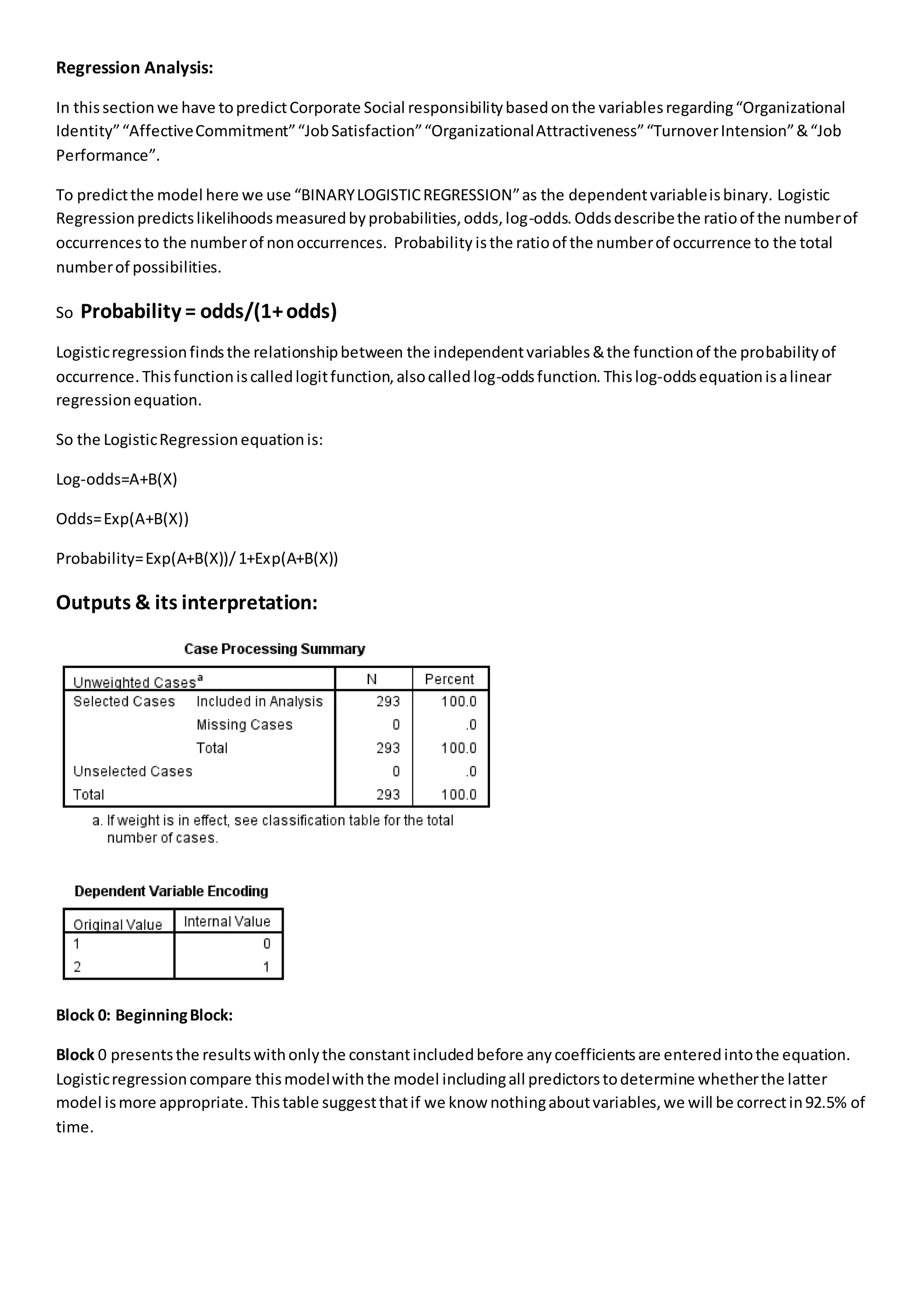
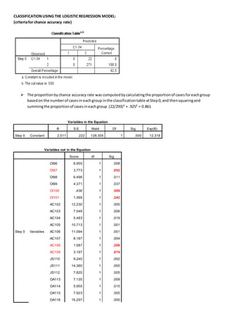
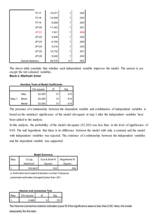
The document discusses a regression analysis aimed at predicting corporate social responsibility using logistic regression based on multiple independent variables. Key elements include the relationship between the variables, model accuracy, and the statistical significance of predictors, which support the existence of a relationship between independent and dependent variables. The logistic regression results indicate good model fit and high classification accuracy rates for predicting group membership.

1. Regression Analysis:
In thissectionwe have topredictCorporate Social responsibilitybasedonthe variablesregarding“Organizational
Identity”“AffectiveCommitment”“JobSatisfaction”“OrganizationalAttractiveness”“TurnoverIntension”&“Job
Performance”.
To predictthe model here we use “BINARYLOGISTICREGRESSION”as the dependentvariableisbinary. Logistic
Regressionpredictslikelihoodsmeasuredbyprobabilities,odds,log-odds. Oddsdescribethe ratioof the numberof
occurrencesto the numberof nonoccurrences. Probability isthe ratioof the numberof occurrence to the total
numberof possibilities.
So Probability = odds/(1+odds)
Logisticregressionfindsthe relationshipbetween the independentvariables&the functionof the probabilityof
occurrence. Thisfunctioniscalledlogitfunction,alsocalledlog-oddsfunction. Thislog-oddsequationisalinear
regressionequation.
So the LogisticRegressionequationis:
Log-odds=A+B(X)
Odds=Exp(A+B(X))
Probability=Exp(A+B(X))/1+Exp(A+B(X))
Outputs & its interpretation:
Block 0: BeginningBlock:
Block 0 presentsthe resultswithonlythe constantincludedbefore anycoefficientsare enteredintothe equation.
Logisticregressioncompare thismodelwiththe model includingall predictorstodetermine whetherthe latter
model ismore appropriate.Thistable suggestthatif we know nothingaboutvariables,we will be correctin92.5% of
time.

2. CLASSIFICATIONUSING THE LOGISTICREGRESSION MODEL:
(criteriafor chance accuracy rate)
 The proportionbychance accuracy rate was computedbycalculatingthe proportionof casesforeachgroup
basedon the numberof casesin eachgroup inthe classificationtable atStep0,and thensquaringand
summingthe proportionof casesineachgroup (22/293)² + .925² = 0.861
Variables not in the Equation
Score df Sig.
Step 0 Variables
OI96 6.955 1 .008
OI97 3.773 1 .052
OI98 6.498 1 .011
OI99 4.371 1 .037
OI100 .436 1 .509
OI101 1.369 1 .242
AC102 12.230 1 .000
AC103 7.549 1 .006
AC104 5.483 1 .019
AC105 10.713 1 .001
AC106 11.094 1 .001
AC107 8.187 1 .004
AC108 1.587 1 .208
AC109 3.197 1 .074
JS110 9.240 1 .002
JS111 14.360 1 .000
JS112 7.820 1 .005
OA113 7.135 1 .008
OA114 5.955 1 .015
OA115 7.923 1 .005
OA116 16.297 1 .000
Variables in the Equation
B S.E. Wald Df Sig. Exp(B)
Step 0 Constant 2.511 .222 128.305 1 .000 12.318

3. TI117 15.071 1 .000
TI118 14.048 1 .000
TI119 8.268 1 .004
JP120 11.342 1 .001
JP121 1.541 1 .214
JP122 5.408 1 .020
JP123 6.769 1 .009
JP124 5.016 1 .025
JP125 10.732 1 .001
JP126 9.046 1 .003
Overall Statistics 58.578 31 .002
The above table conclude that whether each independent variable improves the model. The answer is yes
except the red coloured variables.
Block 1: Method= Enter
Omnibus Tests of Model Coefficients
Chi-square df Sig.
Step 1
Step 52.283 31 .010
Block 52.283 31 .010
Model 52.283 31 .010
The presence of a relationship between the dependent variable and combination of independent variables is
based on the statistical significance of the model chi-square at step 1 after the independent variables have
been added to the analysis.
In this analysis, the probability of the model chi-square (52.283) was less than to the level of significance of
0.05. The null hypothesis that there is no difference between the model with only a constant and the model
with independent variables was rejected. The existence of a relationship between the independent variables
and the dependent variable was supported.
Model Summary
Step -2 Log
likelihood
Cox & Snell R
Square
Nagelkerke R
Square
1 103.943a
.163 .395
a. Estimation terminated atiteration number 7 because
parameter estimates changed byless than .001.
Hosmer and Lemeshow Test
Step Chi-square df Sig.
1 5.466 8 .707
The Hosmer-Lemeshow statistic indicates a poor fit if the significance value is less than 0.05. Here, the model
adequately fits the data.

4. Contingency Table for Hosmer and Lemeshow Test
C1-34 = 1 C1-34 = 2 Total
Observed Expected Observed Expected
Step 1
1 11 12.523 18 16.477 29
2 4 4.521 25 24.479 29
3 5 2.285 24 26.715 29
4 1 .977 28 28.023 29
5 1 .539 29 29.461 30
6 0 .353 29 28.647 29
7 0 .038 4 3.962 4
8 0 .505 55 54.495 55
9 0 .205 29 28.795 29
10 0 .054 30 29.946 30
Next interpretation is for variable in equation. The Exp(B) column presents the extents to which raising the
corresponding measure by one unit influences the odds ratio. If the value exceeds 1 then the odds of an
outcome occurring increase, if it less than 1 ,any increase in the predictor leads to a drop in the odds of the
outcome occurring.
The B values are the Logistic coefficients that can be used to create a predictive equation:
Probability=
𝑒{−2.361+( 𝑂𝐼96×.674)+( 𝑂𝐼95×.118)….}
1+𝑒{−2.361+( 𝑂𝐼96×.674)+( 𝑂𝐼95×.118)… }
The waldstatistic& associatedprobabilitiesprovide anindex of the significance of eachpredictorinthe equation.If
the waldstatisticvalue lessthan.05 rejectthe null hypothesisthatthe variable doesmake asignificantcontribution.

5. Multicollinearityinthe logisticregressionsolutionisdetectedbyexaminingthe standarderrorsforthe b
coefficients.A standarderrorlargerthan2.0 indicatesmulticollinearity amongthe independentvariables.
None of the independentvariablesinthisanalysishadastandarderror largerthan 2.0. The checkfor standarderrors
largerthan 2.0 doesnotinclude the standarderrorfor the Constant.
CLASSIFICATIONUSING THE LOGISTICREGRESSION MODEL:
(criteriaforclassificationaccuracy)

6.  The classificationaccuracyrate should be 25% or more highthan the proportional bychance accuracy rate.
 The accuracy rate computedbySPSSwas93.5% whichwas greaterthan 8.59% the proportional bychance
accuracy rate.
 The value producedbylogisticregressionisaprobabilityvaluebetween 0.0and 1.0.
 The probabilityforgroupmembershipinthe modeledcategoryisabove the cutpoint0.50, the subjectis
predictedtobe a memberof the modeledgroup i.e.group2. If the probabilityisbelow the cutpoint,the
subjectispredictedtobe a memberof the othergroup i.e.group1.
Miss classification list:
MODIFY THE ABOVEMODEL:
HERE WE INCLUDE SECLECTED VARIABLESWHICHMODIFY THE ABOVEMODEL & SATISFYALL CONDITIONS
OF BINARYLOGISTICREGRESSION MODEL. .i.e.
I) OMNIBUS TEST OF MODEL COEFFICIENT(PROBABILITYOFMODEL CHI-SQUARE ≤ 0.05)
II) HOSMER & LEMESHOW TEST(HIGH SIGNIFICANCEVALUEIMPLY GOOD FIT)
III) CLASSIFICATION ACCURACYRATEGREATER THAN PREVIOUS.
NOW THE SELECTED VARIABLESARE: OI96 OI98 OI99 AC102 AC106 JS111 OA114 OA115 OA116 TI117
JP120 JP122 JP123 JP125 JP126 AC108 OI100 OI101 AC109 JP121
Casewise Listb
Case Selected
Statusa
Observed Predicted Predicted Group Temporary Variable
C1-34 Resid ZResid
28 S 1** .975 2 -.975 -6.206
37 S 1** .918 2 -.918 -3.348
121 S 1** .936 2 -.936 -3.811
233 S 1** .930 2 -.930 -3.637
236 S 1** .982 2 -.982 -7.305
240 S 1** .815 2 -.815 -2.097
250 S 1** .863 2 -.863 -2.515
267 S 1** .784 2 -.784 -1.908
269 S 1** .929 2 -.929 -3.609
288 S 1** .909 2 -.909 -3.157
a. S = Selected,U = Unselected cases,and ** = Misclassified cases.
b. Cases with studentized residuals greater than 2.000 are listed.

7. OUTPUT & INTERPRETATION:
Dependent Variable Encoding
Original Value Internal Value
1 0
2 1
Block 0: Beginning Block
Block 0 presentsthe resultswithonlythe constantincludedbefore anycoefficientsare enteredintothe equation.
Logisticregressioncompare thismodelwiththe model includingall predictorstodetermine whetherthe latter
model ismore appropriate. Thistable suggestthatif we know nothingaboutvariables,we will be correctin92.5% of
time.
 The proportionbychance accuracy rate was computedbycalculatingthe proportionof casesforeachgroup
basedon the numberof casesin eachgroup inthe classificationtable atStep0,and thensquaringand
summingthe proportionof casesineachgroup (22/293)² + .925² = 0.861
Variables in the Equation
B S.E. Wald df Sig. Exp(B)
Step 0 Constant 2.511 .222 128.305 1 .000 12.318
Case Processing Summary
Unweighted Casesa
N Percent
Selected Cases
Included in Analysis 293 100.0
Missing Cases 0 .0
Total 293 100.0
Unselected Cases 0 .0
Total 293 100.0
a. If weightis in effect, see classification table for the total number
of cases.

8. Variables not in the Equation
Score df Sig.
Step 0
Variables
OI96 6.955 1 .008
OI98 6.498 1 .011
OI99 4.371 1 .037
AC102 12.230 1 .000
AC106 11.094 1 .001
JS111 14.360 1 .000
OA114 5.955 1 .015
OA115 7.923 1 .005
OA116 16.297 1 .000
TI117 15.071 1 .000
JP120 11.342 1 .001
JP122 5.408 1 .020
JP123 6.769 1 .009
JP125 10.732 1 .001
JP126 9.046 1 .003
AC108 1.587 1 .208
OI100 .436 1 .509
OI101 1.369 1 .242
AC109 3.197 1 .074
JP121 1.541 1 .214
Overall Statistics 57.135 20 .000
The above table conclude that whether each independent variable improves the model. The answer is Yes.
Block 1: Method = Enter
Omnibus Tests of Model Coefficients
Chi-square df Sig.
Step 1
Step 50.636 20 .000
Block 50.636 20 .000
Model 50.636 20 .000
The presence of a relationship between the dependent variable and combination of independent variables is
based on the statistical significance of the model chi-square at step 1 after the independent variables have
been added to the analysis.
In this analysis, the probability of the model chi-square (50.636) was less than to the level of significance of
0.05. The null hypothesis that there is no difference between the model with only a constant and the model
with independent variables was rejected. The existence of a relationship between the independent variables
and the dependent variable was supported.

9. Model Summary
Step -2 Log
likelihood
Cox & Snell R
Square
Nagelkerke R
Square
1 105.591a
.159 .384
a. Estimation terminated at iteration number 7 because
parameter estimates changed byless than .001.
The Hosmer-Lemeshow statistic indicates a poor fit if the significance
value is less than 0.05. Here, the model adequately fits the data.
Contingency Table for Hosmer and Lemeshow Test
C1-34 = 1 C1-34 = 2 Total
Observed Expected Observed Expected
Step 1
1 11 12.435 18 16.565 29
2 5 4.498 24 24.502 29
3 3 2.125 26 26.875 29
4 2 1.048 30 30.952 32
5 1 .556 28 28.444 29
6 0 .265 19 18.735 19
7 0 .726 61 60.274 61
8 0 .250 29 28.750 29
9 0 .095 36 35.905 36
CLASSIFICATIONUSING THE LOGISTICREGRESSION MODEL:
(criteriaforclassificationaccuracy)
Classification Tablea
Observed Predicted
C1-34 Percentage
Correct1 2
Step 1
C1-34
1 6 16 27.3
2 1 270 99.6
Overall Percentage 94.2
a. The cut value is .500
 The classificationaccuracy rate shouldbe 25% or more highthan the proportional bychance accuracy rate.
 The accuracy rate computedbySPSSwas94.2% whichwas greaterthan 9.41% the proportional bychance
accuracy rate.
 The value producedbylogisticregressionisaprobabilityvaluebetween0.0and 1.0.
 The probabilityforgroupmembershipinthe modeledcategoryisabove the cutpoint0.50, the subjectis
predictedtobe a memberof the modeledgroup i.e.group2. If the probabilityisbelow the cutpoint,the
subjectispredictedtobe a memberof the othergroup i.e.group1.
Hosmer and Lemeshow Test
Step Chi-square df Sig.
1 3.349 7 .851

10. Next interpretation is for variable in equation :
The Exp(B) column presents the extents to which raising the corresponding measure by one unit
influences the odds ratio. If the value exceeds 1 then the odds of an outcome occurring increase, if it
less than 1 ,any increase in the predictor leads to a drop in the odds of the outcome occurring.
The B values are the Logistic coefficients that can be used to create a predictive equation:
Probability=
𝑒{−1.977+( 𝑂𝐼96×.713)+( 𝑂𝐼98×.554)….}
1+𝑒{−1.977+( 𝑂𝐼96×.713)+( 𝑂𝐼98×.554)… }
The waldstatistic& associatedprobabilities provide anindex of the significance of eachpredictorinthe
equation.If the waldstatisticvalue lessthan.05 rejectthe null hypothesisthatthe variable doesmake a
significantcontribution.
Variables in the Equation
B S.E. Wald df Sig. Exp(B)
Step 1a
OI96 .713 .404 3.121 1 .077 2.040
OI98 .554 .323 2.948 1 .086 1.740
OI99 .665 .594 1.254 1 .263 1.944
AC102 .622 .309 4.041 1 .044 1.862
AC106 .347 .214 2.625 1 .105 1.414
JS111 .287 .182 2.467 1 .116 1.332
OA114 -.744 .573 1.688 1 .194 .475
OA115 -.499 .724 .476 1 .490 .607
OA116 1.122 .562 3.987 1 .046 3.071
TI117 .394 .265 2.213 1 .137 1.483
JP120 .703 .406 2.993 1 .084 2.019
JP122 -1.240 .844 2.159 1 .142 .289
JP123 .535 .662 .653 1 .419 1.708
JP125 .420 .432 .946 1 .331 1.522
JP126 .590 .613 .926 1 .336 1.804
AC108 -.250 .281 .791 1 .374 .779
OI100 -1.525 .584 6.824 1 .009 .218
OI101 -.551 .438 1.580 1 .209 .576
AC109 -.407 .277 2.154 1 .142 .666
JP121 -.635 .539 1.390 1 .238 .530
Constant -1.977 2.496 .627 1 .428 .139
a. Variable(s) entered on step 1: OI96, OI98, OI99, AC102, AC106, JS111,OA114, OA115,
OA116, TI117, JP120, JP122, JP123, JP125,JP126, AC108, OI100, OI101, AC109, JP121.

11. Multi-colinearity inthe logisticregressionsolutionisdetectedbyexaminingthe standarderrorsforthe b
coefficients.A standarderrorlargerthan2.0 indicatesmulti-colinearity amongthe independentvariables.
None of the independentvariablesinthisanalysishad astandarderror largerthan 2.0. The checkfor standarderrors
largerthan 2.0 doesnotinclude the standarderrorfor the Constant.
Missclassificationlist:
Casewise Listb
Case Selected
Statusa
Observed Predicted Predicted Group Temporary Variable
C1-34 Resid ZResid
6 S 1** .840 2 -.840 -2.289
28 S 1** .969 2 -.969 -5.613
37 S 1** .903 2 -.903 -3.047
121 S 1** .932 2 -.932 -3.705
233 S 1** .959 2 -.959 -4.848
236 S 1** .978 2 -.978 -6.684
240 S 1** .851 2 -.851 -2.387
250 S 1** .817 2 -.817 -2.111
267 S 1** .837 2 -.837 -2.264
269 S 1** .940 2 -.940 -3.976
288 S 1** .898 2 -.898 -2.967
a. S = Selected,U = Unselected cases,and ** = Misclassified cases.
b. Cases with studentized residuals greater than 2.000 are listed.