Classification Algortyhm of Machine Learning

• Logistic Regression
Classification Unlocked

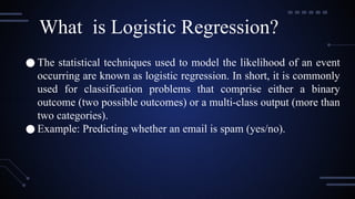
● The statistical techniques used to model the likelihood of an event
occurring are known as logistic regression. In short, it is commonly
used for classification problems that comprise either a binary
outcome (two possible outcomes) or a multi-class output (more than
two categories).
● Example: Predicting whether an email is spam (yes/no).
What is Logistic Regression?

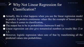
● Actually, this is what happens when you use the linear regression model
to predict. It predicts continuous values like the example of house prices.
But when it comes to classification,
● The output has to be in probabilities (between 0 and 1).
● Linear regression can also give nonsensical numbers as results like -2 or
1.5.
● However, logistic regression takes care of that by transforming all the
predicted values into probabilities.
 Why Not Linear Regression for
Classification?

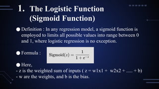
● Definition : In any regression model, a sigmoid function is
employed to limits all possible values into range between 0
and 1, where logistic regression is no exception.
● Formula :
● Here,
- z is the weighted sum of inputs ( z = w1x1 + w2x2 + ..... + b)
- w are the weights, and b is the bias.
1. The Logistic Function
(Sigmoid Function)

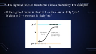
● The sigmoid function transforms into a probability. For example:
𝑧
- If the sigmoid output is close to 1 → the class is likely "yes."
- If close to 0 → the class is likely "no."

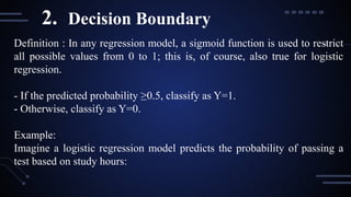
Definition : In any regression model, a sigmoid function is used to restrict
all possible values from 0 to 1; this is, of course, also true for logistic
regression.
- If the predicted probability ≥0.5, classify as Y=1.
- Otherwise, classify as Y=0.
Example:
Imagine a logistic regression model predicts the probability of passing a
test based on study hours:
2. Decision Boundary

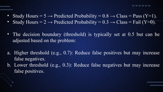
• Study Hours = 5 → Predicted Probability = 0.8 → Class = Pass (Y=1).
• Study Hours = 2 → Predicted Probability = 0.3 → Class = Fail (Y=0).
• The decision boundary (threshold) is typically set at 0.5 but can be
adjusted based on the problem:
a. Higher threshold (e.g., 0.7): Reduce false positives but may increase
false negatives.
b. Lower threshold (e.g., 0.3): Reduce false negatives but may increase
false positives.

● The cost function really measures how well or poorly the model
predicts the labels. In reality, since it is logistic regression, there will be
no mean squared error as in linear regression. That's because:
1. Sigmoid output is non-linear.
2. MSE will create a non-convex cost function and will not have a simple
optimization.
● The Log Loss (Binary Cross-Entropy) Cost Function:
3. Cost Function

Here:
●
𝑦𝑖 : True label (0 or 1).
● y^
𝑖: Predicted probability.
● When the predicted probability is anywhere near the true label (for
example, ^=0.9 for y=1), the loss is minor.
𝑦
● When predicted probability is much much too far from the true
label (for instance, it's ^=0.1 for y=1), penalty extricates.
𝑦
● And such a legend would prod the model to make predictions at
probabilities as near as possible to the true labels.

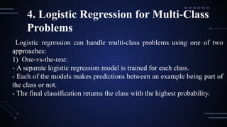
4. Logistic Regression for Multi-Class
Problems
Logistic regression can handle multi-class problems using one of two
approaches:
1) One-vs-the-rest:
- A separate logistic regression model is trained for each class.
- Each of the models makes predictions between an example being part of
the class or not.
- The final classification returns the class with the highest probability.

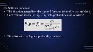
2) Softmax Function:
• This function generalizes the sigmoid function for multi-class problems.
• Converts raw scores ( z1, z2, .... zk) into probabilities for classes
𝑘 :
• The class with the highest probability is chosen.

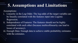
5. Assumptions and Limitations
Assumptions:
i. Linearity in the Log-Odds: The log-odds of the target variable can
be linearly correlated with the features input into Logistic
Regression.
ii. Independence of Features: The features should not be highly
correlated with each other (because multicollinearity can lead to
losses of accuracy).
iii. Enough Data: Enough data to achieve stable probability estimates
with the estimates.

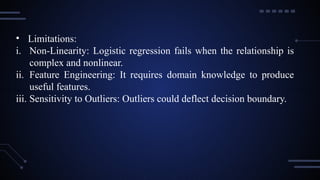
• Limitations:
i. Non-Linearity: Logistic regression fails when the relationship is
complex and nonlinear.
ii. Feature Engineering: It requires domain knowledge to produce
useful features.
iii. Sensitivity to Outliers: Outliers could deflect decision boundary.

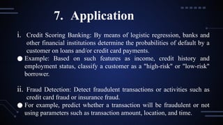
i. Credit Scoring Banking: By means of logistic regression, banks and
other financial institutions determine the probabilities of default by a
customer on loans and/or credit card payments.
● Example: Based on such features as income, credit history and
employment status, classify a customer as a "high-risk" or "low-risk"
borrower.
ii. Fraud Detection: Detect fraudulent transactions or activities such as
credit card fraud or insurance fraud.
● For example, predict whether a transaction will be fraudulent or not
using parameters such as transaction amount, location, and time.
7. Application

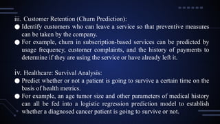
iii. Customer Retention (Churn Prediction):
● Identify customers who can leave a service so that preventive measures
can be taken by the company.
● For example, churn in subscription-based services can be predicted by
usage frequency, customer complaints, and the history of payments to
determine if they are using the service or have already left it.
iv. Healthcare: Survival Analysis:
● Predict whether or not a patient is going to survive a certain time on the
basis of health metrics.
● For example, an age tumor size and other parameters of medical history
can all be fed into a logistic regression prediction model to establish
whether a diagnosed cancer patient is going to survive or not.

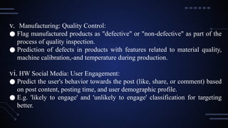
v. Manufacturing: Quality Control:
● Flag manufactured products as "defective" or "non-defective" as part of the
process of quality inspection.
● Prediction of defects in products with features related to material quality,
machine calibration,-and temperature during production.
vi. HW Social Media: User Engagement:
● Predict the user's behavior towards the post (like, share, or comment) based
on post content, posting time, and user demographic profile.
● E.g. 'likely to engage' and 'unlikely to engage' classification for targeting
better.

Classification Unlocked: From
Logistic to Decision Trees
• Support Vector Machine

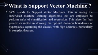
• SVM stands for Support Vector Machines. This is among the
supervised machine learning algorithms that are employed to
perform tasks of classification and regression. This algorithm has
proved its mettle in drawing the optimal decision boundaries or
hyperplanes separating the classes, with high accuracy, particularly
in complex datasets.
What is Support Vector Machine ?

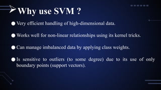
● Very efficient handling of high-dimensional data.
● Works well for non-linear relationships using its kernel tricks.
● Can manage imbalanced data by applying class weights.
● Is sensitive to outliers (to some degree) due to its use of only
boundary points (support vectors).
Why use SVM ?

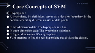
a) Hyperplane :
● A hyperplane, by definition, serves as a decision boundary in the
domain separating different classes of data points.
● In two-dimension data: The hyperplane is a line.
● In three-dimension data: The hyperplane is a plane.
● In higher dimensions: It's a hyperplane.
● SVM attempts to find the best hyperplane that divides the classes.
 Core Concepts of SVM

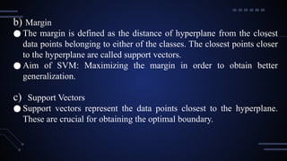
b) Margin
● The margin is defined as the distance of hyperplane from the closest
data points belonging to either of the classes. The closest points closer
to the hyperplane are called support vectors.
● Aim of SVM: Maximizing the margin in order to obtain better
generalization.
c) Support Vectors
● Support vectors represent the data points closest to the hyperplane.
These are crucial for obtaining the optimal boundary.

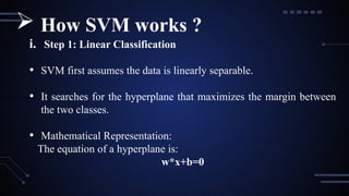
i. Step 1: Linear Classification
• SVM first assumes the data is linearly separable.
• It searches for the hyperplane that maximizes the margin between
the two classes.
• Mathematical Representation:
The equation of a hyperplane is:
w*x+b=0
 How SVM works ?

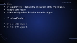
• Here,
• w: Weight vector (defines the orientation of the hyperplane).
• x: Input data vector.
• b: Bias term (defines the offset from the origin).
• For classification:
• If w x+b>0: Class 1.
⋅
• If w x+b<0: Class 0.
⋅

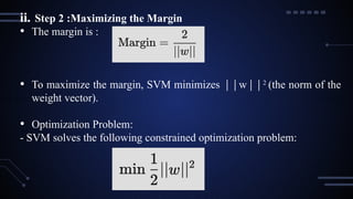
ii. Step 2 :Maximizing the Margin
• The margin is :
• To maximize the margin, SVM minimizes w
∣∣ ∣∣2
(the norm of the
weight vector).
• Optimization Problem:
- SVM solves the following constrained optimization problem:

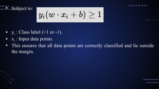
• Subject to:
• yi : Class label (+1 or -1).
• xi : Input data points.
• This ensures that all data points are correctly classified and lie outside
the margin.

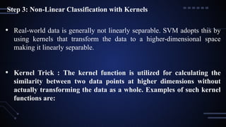
Step 3: Non-Linear Classification with Kernels
• Real-world data is generally not linearly separable. SVM adopts this by
using kernels that transform the data to a higher-dimensional space
making it linearly separable.
• Kernel Trick : The kernel function is utilized for calculating the
similarity between two data points at higher dimensions without
actually transforming the data as a whole. Examples of such kernel
functions are:

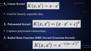
1. Linear Kernel :
• Used for linearly separable data.
2. Polynomial Kernel :
• Captures polynomial relationships.
3. Radial Basis Function (RBF) Kernel (Gaussian Kernel) :

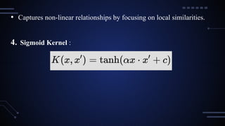
• Captures non-linear relationships by focusing on local similarities.
4. Sigmoid Kernel :

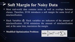
• Most real-world data contains noise as well as overlaps between
classes. Therefore, SVM introduces a soft margin for some level of
misclassification.
• Slack Variables ( ):
𝜉
𝑖 Slack variables are indicators of the amount of
misclassification. SVM minimizes the amount of misclassification
and, at the same time, maximizes the margin.
• Modified Optimization Problem:
 Soft Margin for Noisy Data

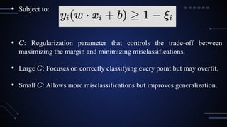
• Subject to:
• 𝐶: Regularization parameter that controls the trade-off between
maximizing the margin and minimizing misclassifications.
• Large : Focuses on correctly classifying every point but may overfit.
𝐶
• Small : Allows more misclassifications but improves generalization.
𝐶

• SVM is primarily a binary classifier but can handle multi-class
problems using:
a) One-vs-One (OvO):
• Builds a classifier for every pair of classes.
• For k classes, it builds k(k−1)/2 classifiers.
• The class with the most "votes" is selected.
b) One-vs-Rest (OvR):
• Builds one classifier for each class vs. the rest.
• The class with the highest confidence score is selected.

i. Effectively working in very high dimensions: Good for datasets with a
large number of dimensions.
ii. Memory Efficient: It will use only the support vectors to represent the
decision boundary.
iii.Versatility: Linear and non-linear relationships can be modeled using
kernels.
iv. Robustness: Not overly sensitive to overfitting, especially with an
appropriate kernel and regularization.
Advantages of SVM

a) Text Classification: Spam detection, sentiment analysis, or classifying
of documents.
b) Image Recognition: Classify images (for instance handwritten digits in
MNIST).
c) Medical Diagnosis: Identify diseases (e.g. cancer detection via patient
data).
d) Fraud Detection: Identify any activity anomaly in banking and e-
commerce.
Applications of SVM

e) Bioinformatics: Classify the DNA sequences or protein structure.
f) Stock Market Prediction: Predict price movement using past data.

• k- Nearest Neighbour

• K nearest neighbor, or simply kNN, holds upon one of the basic
supervised techniques of machine learning. It can perform classification
which is assigning labels to categories, and regression, which is
predicting continuous outcomes. In fact, the principle is very simple:
similar data tend to lead to similar results an axiom derived from the
idea of proximity in feature space.
 Definition

● kNN is a lazy learning algorithm.
1. It does not create an explicit model during training.
2. It merely stores the training dataset and uses that for prediction.
3. Predictions are made by taking into account either the majority class
(classification) or the mean value (regression) of the k-nearest neighbors
from a query point.
What is k-Nearest Neighbors (kNN)?

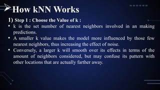
1) Step 1 : Choose the Value of k :
• k is the set number of nearest neighbors involved in an making
predictions.
• A smaller k value makes the model more influenced by those few
nearest neighbors, thus increasing the effect of noise.
• Conversely, a larger k will smooth over its effects in terms of the
amount of neighbors considered, but may confuse its pattern with
other locations that are actually farther away.
How kNN Works

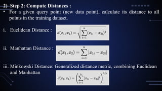
2) Step 2: Compute Distances :
• For a given query point (new data point), calculate its distance to all
points in the training dataset.
i. Euclidean Distance :
ii. Manhattan Distance :
iii. Minkowski Distance: Generalized distance metric, combining Euclidean
and Manhattan

iv. Hamming Distance (for categorical features): Measures the proportion
of mismatched feature values.
3) Step 3 : Identify the k-Nearest Neighbors
• Sort the training data by their distance to the query point.
• Select the k closest points.
4) Step 4: Make a Prediction
• For Classification :
i. Functioning of voting based on majority count among k nearest
neighbours.
ii. Assigning the seeked point to the class which has the highest
occupancy among the mentioned neighbours.

• For Regression:
Compute the average value (mean) of the k nearest neighbors and use it as
the prediction.

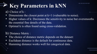
a) Choice of k :
• Dimensions the closest point at k=1 (vulnerable to noise).
• Higher values of k: Decreases the sensitivity to noise but oversmooths
the essential fine details of the data.
• Optimal k is often found using cross-validation.
b) Distance Metric :
• The choice of distance metric depends on the dataset:
• Euclidean distance is the default for continuous data.
• Hamming distance works well for categorical data.
 Key Parameters in kNN

c) Feature scaling :
• All features should be scaled, for instance, via min to max or
standardization, to give equal contribution to the distance calculation.
• If no scaling has been applied, larger ranges of features will dominate
the distance metric.

● Data scalabilitiy: Better accuracy of kNN when the training data is
increasing which shows good representation of neighborhood.
● Non-Linear Flexibility: Effectively deals with complex datasets
having non-linear class boundaries and doesn't require advanced
modelling.
● Incremental Updating: Incorporates new data easily to update to be
included in the already training set without the aid of re-training.
● No Training Overhead: No trainings, it works directly on stored data
for prediction.
 Advantages of KNN

● Medical Diagnosis: Predict diseases according to the accompanying
symptoms, test results, and medical history of patients.
● For example: Classify tumors into benign or malignant.
● Recommender Systems: Suggest products, movies, music on the basis
of preferences of similar users.
● For example, "People who liked this also liked that."
● Image Recognition: Classify images through a comparison in pixel
values to a dataset containing images with labeling.
● Example: Recognition of handwritten digits (e.g., MNIST dataset).
 Applications of KNN

● Text Classification: Organizing documents ranging from spam email
detection to sentiment analysis.
● Example: Emails could be classified based on weightage of words into
either spam or not spam.
● Customer Segmentation: Cluster customers showing similarity in
purchasing behavior for effective targeted marketing campaigns.
● Fraud detection: Recognize abnormal conduct in transactions which
shows sign of the fraud.

 Naive Bayes
Classification Unlocked: From Logistic to
Decision Trees

• Naive Bayes is a family of simple yet powerful supervised machine
learning algorithms that are based on Bayes' Theorem. These have
formed the basis of classification tasks especially in input forms such
as textual documents (spam filtering, sentiment analyses) and
categorical data. Naive Bayes, though simple, regularly matches
complex algorithms.
• Naive Bayes assumes:
◦ Conditional Independence: All features are independent of each other,
given the class label.
◦ Probabilistic Approach: Predictions are based on the probability of a
class label given the feature values.
What is Naive Bayes ?

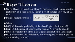
● Naive Bayes is based on Bayes’ Theorem, which describes the
probability of a class label (C) given a set of features (X = x1, x2, ....,
xn).
● Bayes Theorem Formula :
● Where:
● P(C X): Posterior probability of the class C, given the features X.
∣
● P(X C): Likelihood of observing the features X, given the class C.
∣
● P(C): Prior probability of the class C (class distribution in the dataset).
● P(X): Evidence or total probability of observing the features X (acts as
a normalizing constant).
Bayes’ Theorem

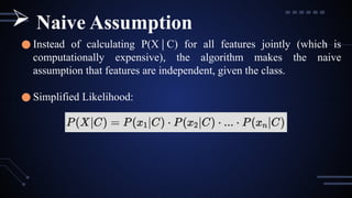
● Instead of calculating P(X C) for all features jointly (which is
∣
computationally expensive), the algorithm makes the naive
assumption that features are independent, given the class.
● Simplified Likelihood:
 Naive Assumption

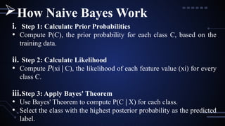
i. Step 1: Calculate Prior Probabilities
• Compute P(C), the prior probability for each class C, based on the
training data.
ii. Step 2: Calculate Likelihood
• Compute (
𝑃 xi∣C), the likelihood of each feature value (xi) for every
class C.
iii.Step 3: Apply Bayes' Theorem
• Use Bayes' Theorem to compute P(C X) for each class.
∣
• Select the class with the highest posterior probability as the predicted
label.
How Naive Bayes Work

i. Gaussian Naive Bayes
● Used for continuous data.
● Assumes features follow a Gaussian (Normal) distribution.
● Likelihood :
● μ: Mean of the feature for class C.
● 𝜎: Standard deviation of the feature for class C.
 Types of Naive Bayes Classifiers

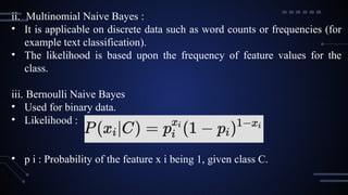
ii. Multinomial Naive Bayes :
• It is applicable on discrete data such as word counts or frequencies (for
example text classification).
• The likelihood is based upon the frequency of feature values for the
class.
iii. Bernoulli Naive Bayes
• Used for binary data.
• Likelihood :
• p i : Probability of the feature x i being 1, given class C.

iv. Complement Naive Bayes
A variation of Multinomial Naive Bayes designed for handling
imbalanced datasets.
Focuses on the probabilities of features not belonging to a class.

● Simplicity: It requires the least time to install and to interpret.
● Scalable: It works most efficiently with large databases, as the model
for frequency computation is direct, involving simple frequency counts.
● Fast Predictions: They are quite inexpensive in terms of computation.
● Effective with Sparse Data: Very effective when performing with sparse
dataset such as term frequencies that represent text.
● Works with Categorical Data: Works most naturally with categorical
kinds of features.
Advantages of Naive Bayes

• Text Classification: Spam detection, sentiment analysis, documentary
categorizing.
• Medical Diagnosis: Predict the diseases from their symptoms and test
results.
• Customer Segmentation: Classify customers into groups based on
behavior or preferences.
• Recommendation Systems: Predict the preferences of users based on
their past activities.
• Fraud Detection: Analyze patterns to identify fraudulent transactions.
 Applications of Naive Bayes

• Decision Tree

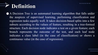
● A Decision Tree is an automated learning algorithm that falls under
the auspices of supervised learning, performing classification and
regression tasks equally well. It takes decision-based splits into a few
subsets according to the values of feature, resulting in a tree-formed
structure. Each decision node indicates a test on a given feature; each
branch represents the outcome of the test, and each leaf node
indicates a class label (in the case of classification) or shows a
continuous value (in the case of regression).
 Definition

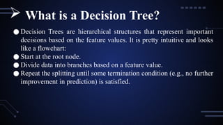
● Decision Trees are hierarchical structures that represent important
decisions based on the feature values. It is pretty intuitive and looks
like a flowchart:
● Start at the root node.
● Divide data into branches based on a feature value.
● Repeat the splitting until some termination condition (e.g., no further
improvement in prediction) is satisfied.
 What is a Decision Tree?

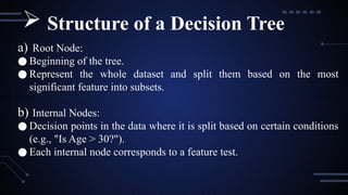
a) Root Node:
● Beginning of the tree.
● Represent the whole dataset and split them based on the most
significant feature into subsets.
b) Internal Nodes:
● Decision points in the data where it is split based on certain conditions
(e.g., "Is Age > 30?").
● Each internal node corresponds to a feature test.
 Structure of a Decision Tree

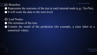
c) Branches:
● Represents the outcome of the test at each internal node (e.g.: Yes/No).
● It will route the data to the next level.
d) Leaf Nodes:
● The terminus of the tree.
● Contain the result of the prediction (for example, a class label or a
numerical value).

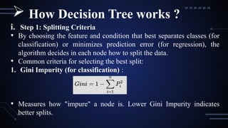
i. Step 1: Splitting Criteria
• By choosing the feature and condition that best separates classes (for
classification) or minimizes prediction error (for regression), the
algorithm decides in each node how to split the data.
• Common criteria for selecting the best split:
1. Gini Impurity (for classification) :
• Measures how "impure" a node is. Lower Gini Impurity indicates
better splits.
 How Decision Tree works ?

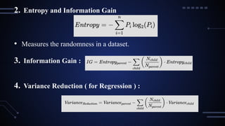
2. Entropy and Information Gain
• Measures the randomness in a dataset.
3. Information Gain :
4. Variance Reduction ( for Regression ) :

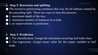
2. Step 2: Recursion and splitting
● The recursive partitioning continues this way for all subsets created by
the preceding split. There are ways to stop this process:
● 1. maximum depth of the tree.
● 2. minimum number of instances in a node.
● 3. no improvement in prediction.
3. Step 3: Prediction
● 1. For classification: Assign the maximum recurring leaf node class.
● 2. For regression: Assign mean value for the target variable in leaf
node.

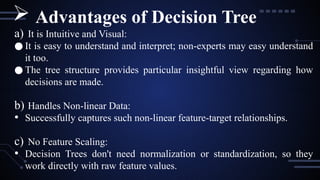
a) It is Intuitive and Visual:
● It is easy to understand and interpret; non-experts may easy understand
it too.
● The tree structure provides particular insightful view regarding how
decisions are made.
b) Handles Non-linear Data:
• Successfully captures such non-linear feature-target relationships.
c) No Feature Scaling:
• Decision Trees don't need normalization or standardization, so they
work directly with raw feature values.
 Advantages of Decision Tree

d) Mixed data type support:
● Works with numerical as well as categorical data without any
additional preprocessing required.
e) Multi-purpose:
● Applicable to classification/regression problems.

i. Pruning:
● Size down the tree by removing superfluous branches.
● It prevents overfitting and improves generalization.
ii. Ensemble Methods:
• Combine different decision trees to improve performance.
a) Random Forest: Combines many trees trained on different subset data
but selected randomly.
b) Gradient Boosting: Each tree is trained sequentially, which then
performs the correction for the errors of the previously constructed tree.
 Techniques to improve Decision Tree

iii.Regularization:
• Limit tree depth by minimum samples per leaf or minimum samples
per split. In this way, overfitting can be avoided.

1. Predictions for Customer Churn:
● Predictions about a customer's departure will be based on his
demographic and behavioral data.
2. Identify Fraud:
● The activity that needs to be caught is whether it can distinguish fraud
on the basis of patterns of transactions.
3. Diagnosis for Medicine:
● Health conditions are classified on the basis of symptoms and tests
associated with these symptoms.
 Application of Decision Tree

4. Scoring Credit:
● Risk for a loan-to-defaulting situation is based on the applicant
information in case of assigning score to an applicant.
5. Market Segmentations:
● Customers need to be split into segments according to consumption.

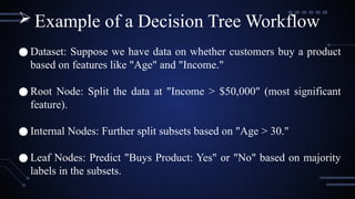
 Example of a Decision Tree Workflow
● Dataset: Suppose we have data on whether customers buy a product
based on features like "Age" and "Income."
● Root Node: Split the data at "Income > $50,000" (most significant
feature).
● Internal Nodes: Further split subsets based on "Age > 30."
● Leaf Nodes: Predict "Buys Product: Yes" or "No" based on majority
labels in the subsets.

Classification Algortyhm of Machine Learning

More Related Content

Similar to Classification Algortyhm of Machine Learning

Recently uploaded

Classification Algortyhm of Machine Learning