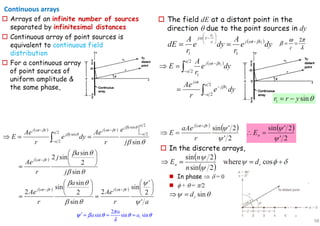
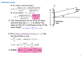
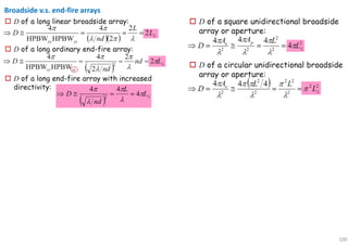
Download as PDF, PPTX


![3
1
[A m s ]
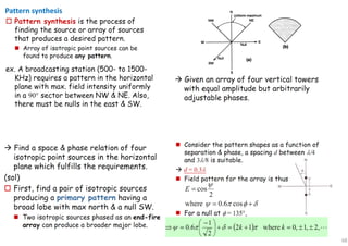
dI dv
L Q
dt dt
−
= ⋅ ⋅
Basic equation of radiation:
2 2
Time-changing current radiates & accelerated charge radiates. or
Radiation is perpendicular to the acceleration. (
( )
Radiated power ( ) or ( ) .
)
LI Qv∝
⊥
i
i
i ɺ ɺ
時變電流 加速電荷都能產生輻射
輻射主要方向 加速度
Radio communication link with Tx antenna & Rx antenna.](https://image.slidesharecdn.com/antennabasic-180827104504/85/Antenna-basic-3-320.jpg)
![6
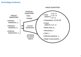
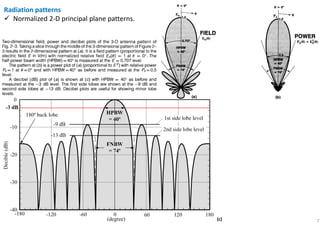
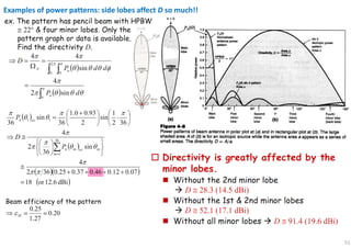
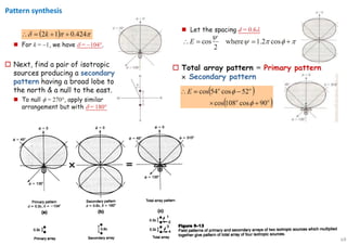
Radiation patterns
To completely specify the radiation pattern with respect to field intensity & polarization, one needs:
1. ( , ) : the -component of the E field as a function of & [V/m].
2. ( , ) : the -component of the E field as a function of & [V/m].
3. ( , ) & ( , ): phase of these fields as a function
E
E
θ
φ
θ φ
θ φ θ θ φ
θ φ φ θ φ
δ θ φ δ θ φ of & [rad or deg].θ φ
max
max
( , )
Normalized field pattern ( , ) [dimsionless]
( , )
Half-power level occurs at those angles & for which ( , ) 1/ 2 0.707.
( , )
Normalized power pattern ( , )
( , )
n
n
n n
E
E
E
E
S
P
S
θ
θ
θ
θ
θ φ
θ φ
θ φ
θ φ θ φ
θ φ
θ φ
θ φ
= =
= =
= =
i
i
10
[dimsionless]
The dB level is given by dB 10log ( , ).nP θ φ=
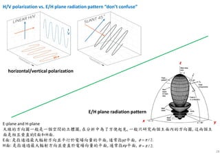
P.S. E-plane and H-plane
天線的方向圖一般是一個空間的立體圖, 在分析中為了方便起見, 一般只研究兩個主面內的方向圖, 這兩個主
面是相互垂直的E面和H面.
E面: 是指通過最大輻射方向並平行於電場向量的平面, 通常指yz平面,
H面: 是指通過最大輻射方向並垂直於電場向量的平面, 通常指xy平面,
/ 2.
/ 2.
φ π
θ π
=
=
x y
z](https://image.slidesharecdn.com/antennabasic-180827104504/85/Antenna-basic-6-320.jpg)
![10
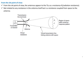
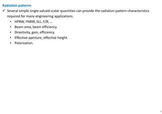
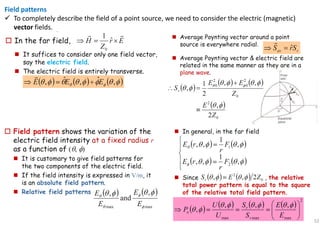
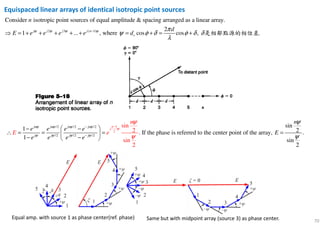
Beam area
2
0 0
4
Beam area of an antenna: ( , )sin ( , ) [sr]
Solid angle through which all the power radiated by the antenna would stream if ( , )
maintained its max. over
A A n nP d d P d
S
φ π θ π
φ θ
π
θ φ θ θ φ θ φ
θ φ
= =
= =
Ω Ω ≡ = Ω∫ ∫ ∫∫i
i
2
max
and was zero elsewhere.
Total radiated power [W].
Beam area of an antenna can be approximated by [sr].
HPBWs in the two principal planes( and planes).
A HP HP
A
AS r
xz yz
θ φΩ
Ω
= Ω
≅
i
i](https://image.slidesharecdn.com/antennabasic-180827104504/85/Antenna-basic-10-320.jpg)
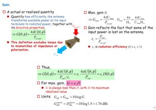
![18
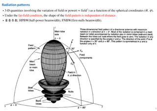
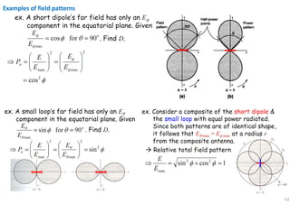
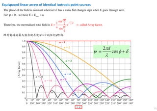
Antenna aperture
* 2
2
Consider a receiving rectangular horn antenna immersed in the field of a uniform plane wave:
1
Poynting vector of the plane wave is Re[ ] [W/m ].
2
Physical aperture of the horn is [m
av
p
P S
A
= = ×E Hi
i
2
].
If horn extracts all the power from the wave over its entire physical aperture,
then the total power absorbed from the wave [W].
However, the field response of the horn is NOT uniform
p p
E
P P SA A
Z
= =
across the aperture.
Effective aperture .
Aperture efficiency .
For horn & parabolic reflector antenna, 0.5 0.8.
e p
e
ap
p
ap
A A
A
A
ε
ε
<
=
≤ ≤
i
i](https://image.slidesharecdn.com/antennabasic-180827104504/85/Antenna-basic-18-320.jpg)
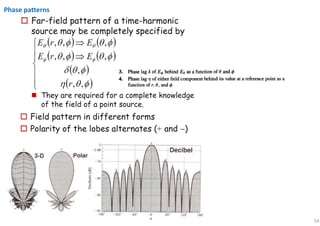
![20
cf:
max max
* 2
4
1. [dimensionless] Directivity from pattern
1
where , Poynting vector of the plane wave is Re[ ] [W/m ].
2
4
2. [dimensionless] Directivity from
av r
r av
A
U U
D
U P
P d Ud P S
D
π
π
≡ =
= ⋅ = Ω = = ×
≡
Ω
∫ ∫avP s E H
2
0 0
4
2
beam area.
where ( , )sin ( , ) [sr]
44
3. [dimensionless] Directivity from aperture.
A n n
e
A
P d d P d
A
D
φ π θ π
φ θ
π
θ φ θ θ φ θ φ
ππ
λ
= =
= =
Ω ≡ = Ω
≡ =
Ω
∫ ∫ ∫∫](https://image.slidesharecdn.com/antennabasic-180827104504/85/Antenna-basic-20-320.jpg)
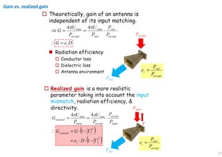
![22
Effective height/aperture
2 22
Relation between the effective height & effective aperture
( / 2)
For an antenna of matched to its load , the power delivered to the load is equal to [W].
4
In terms of the effecti
e
r L
L r
h EV
R R P
R R
= =i
i
2
0
2 20
ve aperture, [W].
[m ].
4
e
e
e e
r
E A
P SA
Z
Z
A h
R
= =
∴ =](https://image.slidesharecdn.com/antennabasic-180827104504/85/Antenna-basic-22-320.jpg)
![30
2
0
0
0
polarization density:
bound volumetric charge dens
[Q/m ]
ity:
where : electric sus
bound surface charge density:
free volumetric charge density:
ceptibility 1,
b
b
e
e r e
ε χ
ε
ε
χ ε χ
ε
ρ
σ
≡ −
=
=
∇
+
≡
+
⋅
= =
⋅ n
P E
D E
a
P
P
P
free surface charge density:
polarization density changes with time, the time-dependent bound-charge density creates a polarization current density
total current density that enter
f
f
t
ρ
σ
≡ ∇⋅
≡ ⋅
∴
∂
=
∂
n
p
D
D a
P
J
s Maxwell's equations is given by
where is the free-charge current density, and the second term is the magnetization current density
also called the bound current density , a contrib( ut) i
t
∂
= + ∇× +
∂
f
f
P
J J M
J
on from atomic-scale magnetic dipoles when they are present.
H-polarization wave , , ( ), magnetic dipoles( )
, .∴
∵當 近地傳播時 會產生極化電流 外加自由電荷 很小 地磁 很小
總電荷密度大小會是上式 產生的熱會使信號迅速衰減
Polarization current detail analysis](https://image.slidesharecdn.com/antennabasic-180827104504/85/Antenna-basic-30-320.jpg)

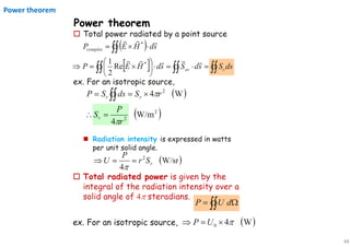
![47
Power patterns
A Tx antenna can be represented by a point source at the origin
• Radiated energy streams out in radial lines.
• Time rate of energy flow per unit area [W/m2].
• Poynting vector has only a radial component.
An isotropic source radiates energy uniformly in all directions.
All antennas have directional properties anisotropic sources
• Absolute power pattern.
• Relative power pattern.
• Normalized power pattern.
ˆ rrS=S](https://image.slidesharecdn.com/antennabasic-180827104504/85/Antenna-basic-47-320.jpg)


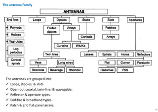
This document discusses various topics related to antenna fundamentals including: 1. It defines key antenna terminology such as radiation patterns, beamwidth, directivity, gain, polarization, and more. 2. It describes different categories of antenna types including loops, dipoles, slots, reflectors, patches, and more. 3. It covers antenna parameters and concepts such as radiation patterns, beam efficiency, radiation intensity, effective aperture, polarization, near and far field zones, and more.


![RF Circuit Design - [Ch4-2] LNA, PA, and Broadband Amplifier](https://cdn.slidesharecdn.com/ss_thumbnails/ch4-2-150613064410-lva1-app6891-thumbnail.jpg?width=640&height=640&fit=bounds)