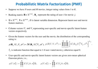
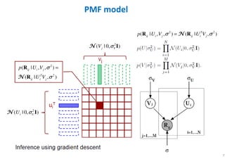
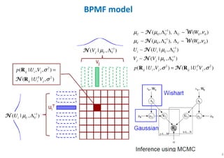
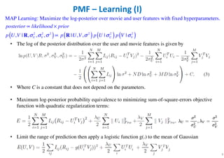
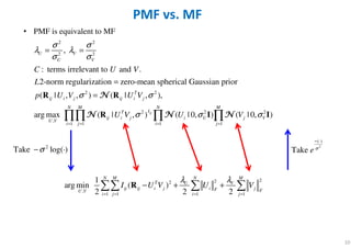
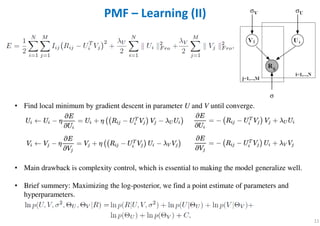
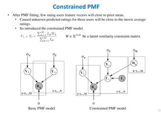
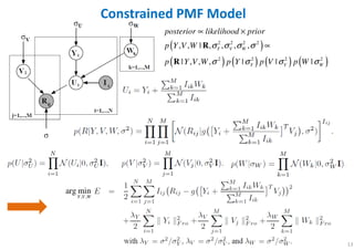
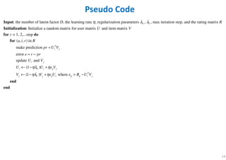
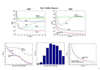
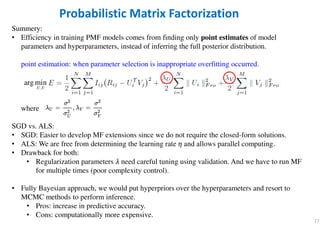
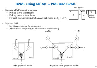
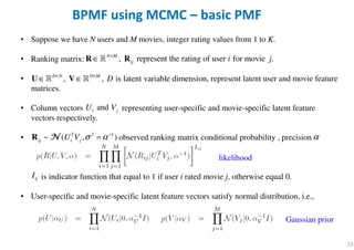
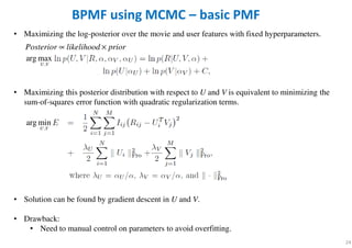
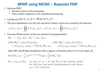
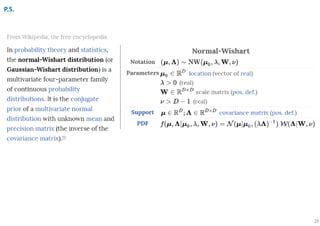
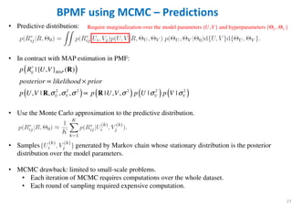
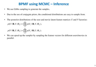
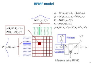
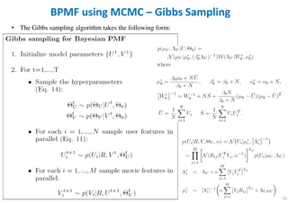
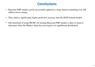
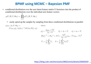
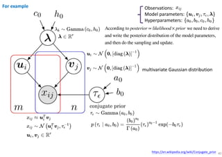
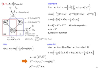
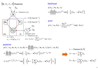
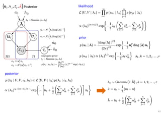
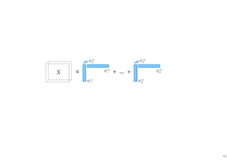
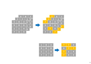
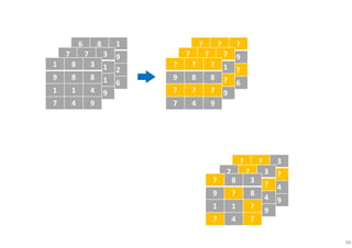
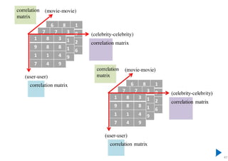
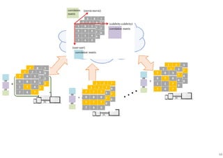
The document outlines probabilistic matrix factorization (PMF) and its applications in recommendation systems, particularly focusing on models like Bayesian PMF (BPMF) and constrained PMF. It discusses the mathematical foundations, learning processes, and comparisons between several factorization methods, emphasizing challenges such as computational complexity and parameter tuning. Additionally, it highlights the advantages of Bayesian approaches in improving predictive accuracy while addressing their computational demands.

1. 1
Dec. 3, 2018
Jay Chang
PMF, BPMF and BPTF

2. Probabilistic Matrix Factorization
(PMF)
2
R. Salakhutdinov and A. Mnih, “Probabilistic Matrix Factorization,” Proc. Advances in Neural Information Processing Systems 20 (NIPS 07), ACM
Press, 2008, pp. 1257-1264.

3. 3
Recommendation = Prediction of Rating
• In real systems, matrix is really big and sparse
• E.g. dataset from Netflix Price: 500,000 users x 17,000 movies.
• 100 million (~1%) ratings are known.

4. 4
Recommendation System – Classification
Tensor
Factorization

5. 5
Preliminaries
• Suppose we have N users and M movies, integer rating values from 1 to K.
• Ranking matrix:
• Represent latent user and movie
feature matrices.
• We will use Ui and Vj to denote the latent feature vectors for user i and movie j respectively.
, represent the rating of user for movie .N M
ij i j×
∈R Rℝ
, , is latent variable dimension.D N D M
D× ×
∈ ∈U Vℝ ℝ

6. 6
Probabilistic Matrix Factorization (PMF)
• Suppose we have N users and M movies, integer rating values from 1 to K.
• Ranking matrix:
• Represent latent user and movie
feature matrices.
• Column vectors representing user-specific and movie-specific latent feature
vectors respectively.
• Given the feature vectors for the user and the movie, the distribution of the corresponding
rating is:
is indicator function that equal to 1 if user i rated movie j, otherwise equal 0.
• User-specific and movie-specific latent feature vectors are given zero-mean spherical
Gaussian priors, i.e.,
, represent the rating of user for movie .N M
ij i j×
∈R Rℝ
, , is latent variable dimension.D N D M
D× ×
∈ ∈U Vℝ ℝ
andi jU V
2 2
( | ) | , ), ( ,, T
i ijj ji ijp UU V V σσ =R RNNNN
ijI

7. 7
2
2
( | )
( | , )
, ,iij j
T
ij i j
U Vp
U V σ
σ =R
RNNNN
2
( | 0, )j VV σ INNNN
2
( | 0, )i UU σ INNNN
2 2
( | ) ( | , ), ,i
T
ij j ij i jU Vp U V σσ =R RNNNN
PMF model

8. 8
BPMF model
2
2
( | )
( | , )
, ,iij j
T
ij i j
U Vp
U V σ
σ =R
RNNNN
1
( | , )j V VV µ −
ΛNNNN
1
( | , )i U UU µ −
ΛNNNN
1
0 0 0
1
0 0 0
2
1
1
2
( , ), ( , )
( , ), ( , )
( | , )
( | , )
( | ) ( |, , ),
U U U
V V V
i i U U
j j V V
T
ij ij ii jj
W
W
U U
U V
V V
p U V
µ µ ν
µ µ ν
µ
µ
σσ
−
−
−
−
Λ Λ ∼
Λ Λ ∼
Λ
Λ
=R R
N WN WN WN W
N WN WN WN W
NNNN
NNNN
NNNN
∼
∼
∼
∼

9. • The log of the posterior distribution over the user and movie features is given by
• Where C is a constant that does not depend on the parameters.
• Maximum log-posterior probability equivalence to minimizing sum-of-square-errors objective
function with quadratic regularization terms:
• Limit the range of prediction then apply a logistic function g(.) to the mean of Gaussian
functions
9
PMF – Learning (I)
( ) ( ) ( ) ( )2 2 2 2 2 2
MAP Learning: Maximize the log-posterior over movie and user features with fixed hyperparameters.
, | , , , | , , | |U V U V
posterior likelihood prior
p U V p U V p U p Vσ σ σ σ σ σ
∝ ×
∝R R

10. 10
PMF vs. MF
• PMF is equivalent to MF
2 2
2
2
,
1 1 1
2
2
2 2
,
: terms irrelevant to and .
2-norm regularization zero-mean spherical Gaussian
, ,
a
prior
( | ) ( | , ),
( | , ) ( | 0, ) ( | 0,rg max ij
i j
N M N
U V
U V
U V
T
ij ij i j
IT
ij i j i U
i j i
j
U
C U V
L
p U V
U V U V
V
σ σ
λ λ
σ σ
σ
σ
σ
σ
= = =
= =
=
=
∏∏ ∏
R R
R I
NNNN
N N NN N NN N NN N N 2
1
)
M
j
Vσ
=
∏ I
,
1 1
22
1 1
21
arg ( )min
2 2 2
N
T
ij ij i j i
M N M
jF
U V
U V
i j i
F
j
I U V U V
λ λ
= = = =
+ +−  R
2
Take log( )σ− ⋅
2
( )
Take e σ
− ⋅

11. • Find local minimum by gradient descent in parameter U and V until converge.
• Main drawback is complexity control, which is essential to making the model generalize well.
• Brief summery: Maximizing the log-posterior, we find a point estimate of parameters and
hyperparameters.
11
PMF – Learning (II)

12. 12
Constrained PMF
• After PMF fitting, few rating users feature vectors will close to prior mean.
• Caused unknown predicted ratings for those users will be close to the movie average
ratings.
• So introduced the constrained PMF model.
Constrained PMF modelBasic PMF model
be a latent similarity constraint matrixD M
W ×
∈ℝ

13. 13
Constrained PMF Model
( )
( ) ( ) ( ) ( )
2 2 2 2
2 2 2 2
, , | , , , ,
| , , , | | |
Y V W
Y V W
posterior likelihood prior
p Y V W
p Y V W p Y p V p W
σ σ σ σ
σ σ σ σ
∝
∝
×
R
R
, ,
arg min
Y V W

14. 14
: the number of latent factor , the learning rata , regularization parameters , , max iteration step, and the rating matrix
: Initialize a random matrix for user matrix and
U VD R
U
λη λInput
Initialization
= 1, 2,...step
( , , ) in
make prediction
error
update and
(1 )
(1 )
item matrix
T
i j
i j
i U i ij j
j V
t
u i r R
pr U V
e r pr
U V
U U e V
V
V
ηλ η
ηλ
=
= −
← − +
← −
for do
for
where T
j ij i ij ij i jV e U e R U Vη+ = −
end
end
Pseudo Code

15. 15
Demo
RMSE
iterations
training set : validation set = 8:2

16. 16

17. 17
Summery:
• Efficiency in training PMF models comes from finding only point estimates of model
parameters and hyperparameters, instead of inferring the full posterior distribution.
point estimation: when parameter selection is inappropriate overfitting occurred.
where
SGD vs. ALS:
• SGD: Easier to develop MF extensions since we do not require the closed-form solutions.
• ALS: We are free from determining the learning rate ߟ and allows parallel computing.
• Drawback for both:
• Regularization parameters ߣ need careful tuning using validation. And we have to run MF
for multiple times (poor complexity control).
• Fully Bayesian approach, we would put hyperpriors over the hyperparameters and resort to
MCMC methods to perform inference.
• Pros: increase in predictive accuracy.
• Cons: computationally more expensive.
Probabilistic Matrix Factorization
,
arg min
U V

18. 18
• R. Salakhutdinov and A. Mnih, “Probabilistic Matrix Factorization,” Proc. Advances in
Neural Information Processing Systems 20 (NIPS 07), ACM Press, 2008, pp. 1257-1264.
• Koren, Y., Bell, R., Volinsky, C. “Matrix factorization techniques for recommender systems”,
Computer, 2009, 42, (8), pp. 30–37.
References

19. 19
Some Derivations for Eq(3)

20. 20
Some Constrained PMF SGD Derivations

21. 21
Bayesian Probabilistic Matrix
Factorization (BPMF) using
Markov Chain Monte Carlo
(MCMC)
R. Salakhutdinov and A. Mnih. “Bayesian probabilistic matrix factorization using Markov chain Monte Carlo”, In International Conference on
Machine learning, pages 880–887, 2008.

22. 22Bayesian PMF graphical modelPMF graphical model
≈R U
V
user features
movie
features
BPMF using MCMC – PMF and BPMF
T
ij i j≈R U V
• Consider a PMF generative process:
• Pick up user u latent factor.
• Pick up movie v latent factor.
• For each (user, movie) pair observed: pick rating as
• Bayesian PMF:
• Introduce priors for the parameters.
• Allow model complexity to be controlled automatically.

23. 23
BPMF using MCMC – basic PMF
• Suppose we have N users and M movies, integer rating values from 1 to K.
• Ranking matrix:
• , represent latent user and movie feature
matrices.
• Column vectors representing user-specific and movie-specific latent feature
vectors respectively.
• observed ranking matrix conditional probability , precision
is indicator function that equal to 1 if user i rated movie j, otherwise equal 0.
• User-specific and movie-specific latent feature vectors satisfy normal distribution, i.e.,
, represent the rating of user for movie .N M
ij i j×
∈R Rℝ
, , is latent variable dimension.D N D M
D× ×
∈ ∈U Vℝ ℝ
andi jU V
2 1
~ ( , )T
ij i jU V σ α−
=R NNNN
likelihood
ijI
Gaussian prior
α

24. • Maximizing the log-posterior over the movie and user features with fixed hyperparameters.
• Maximizing this posterior distribution with respect to U and V is equivalent to minimizing the
sum-of-squares error function with quadratic regularization terms.
• Solution can be found by gradient descent in U and V.
• Drawback:
• Need to manual control on parameters to avoid overfitting.
24
BPMF using MCMC – basic PMF
Posterior likelihood prior∝ ×
,
arg max
U V
,
arg min
U V

25. 25
BPMF using MCMC – Bayesian PMF
• The prior distributions over the user and movie feature vectors are assumed to be Gaussian:
• Gaussian-Wishart priors on the user and movie hyperparameters:
where W is the Wishart distribution with ߥ0 degrees of freedom and a D × D scale matrix W0
• Bayesian PMF:
• Introduce priors for the parameters.
• Allow model complexity to be controlled automatically.
• Likelihood
2 2
( | , , ) ( | , )T
ij i j ij i jp R U V R U Vσ σ= NNNN

26. 26
P.S.

27. • Predictive distribution:
• In contract with MAP estimation in PMF:
27
BPMF using MCMC – Predictions
• Use the Monte Carlo approximation to the predictive distribution.
• Samples generated by Markov chain whose stationary distribution is the posterior
distribution over the model parameters.
• MCMC drawback: limited to small-scale problems.
• Each iteration of MCMC requires computations over the whole dataset.
• Each round of sampling required expensive computation.
( )
( ) ( ) ( ) ( )2 2 2 2 2 2
, | , , , | , , | |
|{ , } ( )ij M
U U V
A
V
P
posterior likelihood prior
p U V p U V
p R U V
p U p Vσ σ σ σ σ σ
∗
∝ ×
∝R R
R
Require marginalization over the model parameters { , } and hyperparameters { , }U VU V Θ Θ

28. 28
• We use Gibbs sampling to generate the samples.
• Due to the use of conjugate priors, the conditional distributions are easy to sample from.
• The posterior distributions of the user and movie latent feature matrices U and V factorize:
• We can speed up the sampler by sampling the feature vectors for different users/movies in
parallel.
BPMF using MCMC – Inference
1
1
( | , , ) ( | , , ),
( | , , ) ( | , , ).
N
U i U
i
N
U j V
j
p U V p U V
p V U p V U
=
=
Θ = Θ
Θ = Θ
∏
∏
R R
R R

29. 29
BPMF model
2
2
( | )
( | , )
, ,iij j
T
ij i j
U Vp
U V σ
σ =R
RNNNN
1
( | , )j V VV µ −
ΛNNNN
1
( | , )i U UU µ −
ΛNNNN
1
0 0 0
1
0 0 0
2
1
1
2
( , ), ( , )
( , ), ( , )
( | , )
( | , )
( | ) ( |, , ),
U U U
V V V
i i U U
j j V V
T
ij ij ii jj
W
W
U U
U V
V V
p U V
µ µ ν
µ µ ν
µ
µ
σσ
−
−
−
−
Λ Λ ∼
Λ Λ ∼
Λ
Λ
=R R
N WN WN WN W
N WN WN WN W
NNNN
NNNN
NNNN
∼
∼
∼
∼

30. 30
BPMF using MCMC – Overall Model
likelihood
Prior ~ Wishart
Prior ~ Normal
Prior ~ Gaussian
approximate posterior
conditional prob ~
Normal-Wishart

31. 31
• The Gibbs sampling algorithm takes the following form:
BPMF using MCMC – Gibbs Sampling

32. 32
Demo
RMSE
iterations
training set : validation set = 9:1

33. 33

34. 34
• Bayesian PMF models can be successfully applied to a large dataset containing over 100
million movie ratings.
• They achieve significantly higher predictive accuracy than the MAP-trained models.
• One drawback of using MCMC for training Bayesian PMF models is that it is hard to
determine when the Markov chain has converged to its equilibrium distribution.
Conclusions

35. 35
• R. Salakhutdinov and A. Mnih. “Bayesian probabilistic matrix factorization using Markov
chain Monte Carlo”, In International Conference on Machine learning, pages 880–887, 2008.
References

36. 36

37. 37

38. 38
P.S. Gibbs sampling = alternating conditional sampling
• 假設觀測值 服從mean(unknown)為 ，covariance(known)為
，且變量ߐ服從均勻分佈，利用Gibbs採樣估計ߐ ?
•
https://en.wikipedia.org/wiki/Conjugate_prior
或是我們也可從joint Gauss求出後驗。
alternating

39. 39
BPMF using MCMC – Bayesian PMF
• conditional distribution over the user latent feature matrix U factorizes into the product of
conditional distributions over the individual user feature vectors.
• easily speed up the sampler by sampling from these conditional distributions in parallel.
https://blog.csdn.net/shenxiaolu1984/article/details/50405659

40. 40https://en.wikipedia.org/wiki/Conjugate_prior
conjugate prior
Observations:
Model parameters:
Hyperparameters:
According to e need to derive
and write the posterior distribution of the model parameters,
and then do the sampling and updat .
w
e
osterior likelihood priorp ×∝
For example
multivariate Gaussian distribution

41. 41
{ }, , ,i j ετ λu v Posterior likelihood
Khatri-Rao product
bij indicator function
prior posterior

42. 42
{ }, , ,i j ε λτu v likelihood
prior
posterior
Posterior

43. 43
{ }, , ,i j ε λτu v likelihood
prior
posterior
Posterior

44. 44
(1)
1U (1)
RU
(2)
RU
(3)
RU
(2)
1U
(3)
RU

45. 45
6 8 1
7 4 9
3 5 2
1 2 6
7 7 3
8 2 1
8 8 1
4 1 9
1 8 3
9 8 8
1 1 4
7 4 9
1 8 3
9 8 8
1 1 4
7 4 9
? ? 3
9 ? ?
? 1 4
? 4 9
? 8 1
7 4 9
3 5 2
1 2 ?
? 7 3
8 2 1
8 8 1
4 1 ?
? 8 3
9 8 8
1 ? 4
7 4 ?

46. 46
6 8 1
7 4 9
3 5 2
1 2 6
7 7 3
8 2 1
8 8 1
4 1 9
1 8 3
9 8 8
1 1 4
7 4 9
? ? ?
7 4 9
3 5 ?
1 2 6
? ? ?
8 2 1
8 8 ?
4 1 9
? ? ?
9 8 8
? ? ?
7 4 9
? ? 3
9 ? ?
? 1 4
? 4 9
7 ? 3
9 ? ?
? 1 4
? 4 9
? 8 3
9 ? 8
1 1 ?
? 4 ?

47. 47
6 8 1
7 4 9
3 5 2
1 2 6
7 7 3
8 2 1
8 8 1
4 1 9
1 8 3
9 8 8
1 1 4
7 4 9
(user-user)
(celebrity-celebrity)
(movie-movie)
correlation matrix
correlation matrix
correlation
matrix

48. 48
or
or
+

49. 49
Five Pillars Of The Mamba Mentality:
1. Be Passionate.
2. Be Obsessive.
3. Be Relentless.
4. Be Resilient.
5. Be Fearless.
“Obsessiveness is having the attention to detail for the action you are performing at the time
you’re performing it.”
“Success is the ability to use your passion to help someone else discover their passion.”
https://www.youtube.com/watch?v=NLElzEJPceA

50. 50https://www.ted.com/talks/linda_hill_how_to_manage_for_collective_creativity

51. 51
Thank you for your attention