Downloaded 26 times


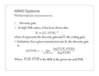


![EE- Trade-
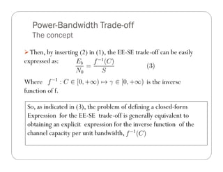
EE-ES Trade-off for MIMO Systems
MIMO Capacity
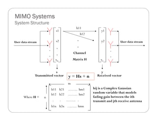
Consider the MIMO-system model
y = Hx + n
With:
o The signal is transmitted over M transmit antennas
and received over N received antennas,
o , is a random matrix having independent and
identically distributed (i.i.d.) complex circular Gaussian
entries with zero-mean and unit variance.
o n: zero–mean complex Gaussian noise. Independent and
equal variance real and imaginary parts. E[nn†] = IN](https://image.slidesharecdn.com/power-bandwidthtradeoff-130206064608-phpapp02/85/The-Power-Bandwidth-Tradeoff-in-MIMO-Systems-19-320.jpg)

![EE- Trade-
EE-ES Trade-off for MIMO Systems
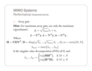
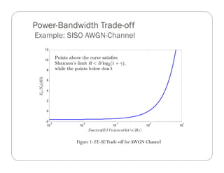
EE-SE Approximations - 1
o In [1], they approximated the EE-SE trade-off for the
situation of low SE and low EE.
o The approximated EE-SE trade-off is expressed as:
(5)
Where donates the minimum required for reliable
communication, and denotes the slope of spectral
efficiency in b/s/Hz/(3 dB) at the point](https://image.slidesharecdn.com/power-bandwidthtradeoff-130206064608-phpapp02/85/The-Power-Bandwidth-Tradeoff-in-MIMO-Systems-22-320.jpg)

![EE- Trade-
EE-ES Trade-off for MIMO Systems
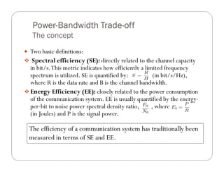
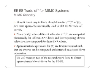
EE-SE Approximations - 2
o In [2], a closed-form approximation is provided for (4), as
follow:
Where
And is the ratio between receive and transmit
antennas
o This approximation was approved to have an acceptable
accuracy for M or N >2](https://image.slidesharecdn.com/power-bandwidthtradeoff-130206064608-phpapp02/85/The-Power-Bandwidth-Tradeoff-in-MIMO-Systems-24-320.jpg)
![EE- Trade-
EE-ES Trade-off for MIMO Systems
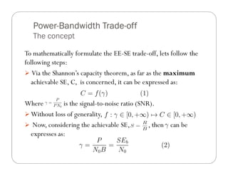
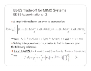
EE-SE Approximations - 2
Case II: M≠N, , then
(7)
Where: ,
and
are values depending on the value of (see table I
in [2])](https://image.slidesharecdn.com/power-bandwidthtradeoff-130206064608-phpapp02/85/The-Power-Bandwidth-Tradeoff-in-MIMO-Systems-26-320.jpg)

![EE- Trade-
EE-ES Trade-off for MIMO Systems
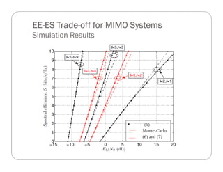
Simulation Results
The following simulation result presented in [2], where the EE-
SE trade-offs is plotted for three methods:
Numerical computation: as mentioned previously using Monte
Carlo simulation to get the inverse of (4).
Using approximation-1 as described in (5), and detailed in [1].
Using approximation-2 as described in (6) and (7) and detailed
in [2].
Results are simulated for different number of transmit (t) and
receive (r) antennas.](https://image.slidesharecdn.com/power-bandwidthtradeoff-130206064608-phpapp02/85/The-Power-Bandwidth-Tradeoff-in-MIMO-Systems-28-320.jpg)

![References
[1] S. Verdu, "Spectral efficiency in the wideband regime", IEEE Trans. Inf. Theory,,
vol. 48, no. 6, pp. 13191343, June 2002
[2] F. Hliot, M. Imran, and R. Tafazolli, "On the Energy efficiency -Spectral efficiency
Trade-o over the MIMO Rayleigh Fading Channel“ ,IEEE Trans. Communications,
VOL. 60, NO. 5, MAY 2012.
[3] I. E. Telatar, "Capacity of multi-antenna Gaussian channels“ ,Europe. Trans.
Telecomm. Related Techno, vol. 10, no. 6, pp. 585596, Nov. 1999.
[4] F. Hliot, M. Imran, and R. Tafazolli, "An accurate closed-form approximation of
the energy efficiency -spectral efficiency trade-o over the MIMO Rayleigh fading
channel“ ,in Proc. 2011 IEEE ICC, 4th Int. Workshop Green Comm..,
[5] O. Oyman and A. J. Paulraj, "Spectral efficiency of relay networks in the power
limited regime",in Proc. 2004 Allerton Conf. Commun., Control Computing.
[6] S. de la Kethulle, "An Overview of MIMO Systems in Wireless
communications," Lecture in Communication Theory for Wireless Channels,
September 27, 2004.](https://image.slidesharecdn.com/power-bandwidthtradeoff-130206064608-phpapp02/85/The-Power-Bandwidth-Tradeoff-in-MIMO-Systems-32-320.jpg)

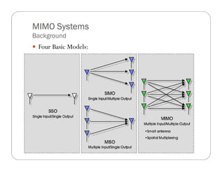
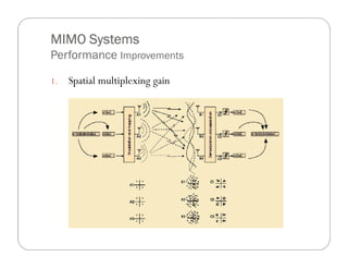
The document discusses the power-bandwidth tradeoff in MIMO systems. It begins with background on MIMO systems, including their structure and key performance improvements like spatial multiplexing gain and diversity gain. It then defines spectral efficiency and energy efficiency, noting that maximizing both is not possible due to the inherent tradeoff between them known as the EE-SE tradeoff. The concept of this tradeoff is explained through mathematical formulations. As an example, the EE-SE tradeoff for an AWGN channel is shown. Approximation methods for determining the EE-SE tradeoff in MIMO systems are also presented.


![[Year 2012-13] Mimo technology](https://cdn.slidesharecdn.com/ss_thumbnails/mimotechnology-180701101303-thumbnail.jpg?width=640&height=640&fit=bounds)