In this paper, I present the MIMO channel for single user case, discuss the decomposition of MIMO into parallel independent channels, and estimate the MIMO channel capacity. Then, I discuss on computation of capacity region for multiuser MIMO broadcast and multiple access channel and plot capacity regions for two users case. I conclude by showing the duality relationship between the multiple access and broadcast channel and show its significance for numerical standpoint.

1. Multiuser MIMO Gaussian Channels:
Capacity Regions and Duality
Shristi Nhuchhe Pradhan
Electrical and Computer Engineering
The University of British Columbia, Vancouver
shristip@ece.ubc.ca
Abstract
Multiple-input and multiple-output or MIMO is one of the smart antenna technologies which
uses multiple transmit and receive antenna for improved communication performance. This field
has been exploited significantly to increase capacity of wireless channels. In this paper, we first
model the MIMO channel for single user case, discuss the decomposition of MIMO into parallel
independent channels and estimate the MIMO channel capacity. We then focus on computation
of capacity region for multiuser MIMO broadcast and multiple access channel and plot capacity
regions for two users case. We conclude by showing the duality relationship between the multiple
access and broadcast channel and show its significance for numerical standpoint.
1 Introduction
Today’s wireless systems support and demand multiusers, but still single-user results are of much
interest. Here, we start with the MIMO channel model for single user case by considering a com-
munication system of Mt transmit and Mr receive antennas which can be represented as [1]:
y = Hx + n (1.1)
1

2. where, y is the Mr dimensional received vector, x is the Mt dimensional transmitted vector, n is the
Mr dimensional noise vector and H is the Mr ⇥ Mt matrix of channel gains. A channel bandwidth
of B and complex Gaussian noise with zero mean and covariance matrix sv2
nIMr , where 2
n = N0B.
1.1 Parallel decomposition of the MIMO channels
The MIMO channel can be decomposed into a number of R parallel independent channels. In
fact, by multiplexing data onto these independent channels, communication system with multiple
antennas at the transmitter and receiver gives an R-fold increase in data rate as compared to those
with just one antenna at the transmitter and receiver side [1].
Consider the MIMO channel as mentioned earlier. We assume that channel is known at both
transmitter and receiver. Let RH denote the rank of H. We can obtain the singular value decom-
position (SVD) of matrix H as [2]:
H = U⌃VH
(1.2)
where U is a Mr ⇥Mr unitary matrix, V is a Mt ⇥Mt unitary matrix and ⌃ is a Mr ⇥Mt diagonal
matrix of singular values { i} of H. Here, svi =
p
i for i the ith eigenvalue of HHH. HH is the
conjugate transpose or Hermitian transpose of H. Also, RH  min(Mt, Mr), as rank cannot be
greater than the number of rows or columns.
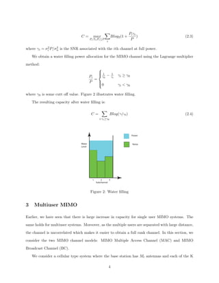
Parallel channels from MIMO system is obtained through transmit precoding on the channel
input x and receiver shaping on the channel output y. In transmit precoding, we obtain the input
to the antennas x through a linear transformation on input vector ˜x as x = VH˜x. Similarly, in
receiver shaping, we multiply the channel output y with UH as ˜y = UHy. This is illustrated in
Figure 1.
Figure 1: Transmit Precoding and Receiver Shaping
Therefore,
˜y = ⌃˜x + ˜n (1.3)
Hence, MIMO channel is decomposed into RH independent parallel channels where the ith
2

3. channel has input ˜xi, output ˜yi, noise ˜n and channel gain and MIMO support RH times the data
rate of a system with just one antenna at the transmitter and receiver. This leads to a multiplexing
gain of RH.
2 MIMO channel capacity
Shannon’s capacity for a MIMO channel gives the maximum rate at which information can be
transmitted over the channel of specified bandwidth in the presence of noise with arbitrarily small
error probability. The channel gain matrix determines the channel capacity. In this paper, we
assume that channel matrix is drawn from an independent identically distributed (i.i.d) Gaussian
distribution and that it is static i.e. time-invariant. The capacity in terms of mutual information
between input x and output y is given as:
C = max
p(x)
I(X; Y ) = max
p(x)
[H(Y) H(Y | X)] (2.1)
where I(X; Y ) is the mutual information between x and y, H(Y) and H(Y | X) is the entropy in
y and y/x. Since Y = X + N and the noise is independent of X, H(Y | X) = H(N), the entropy
of noise. Here, maximizing the mutual information is equivalent to maximizing the entropy in y as
entropy in noise is fixed and independent of the channel input.
As given in [2], the entropy of y is maximized when y is a zero-mean circularly-symmetric
complex Gaussian (ZMCSCG) random variable. Also, y is ZMCSCG only if input x is ZMCSCG,
which is optimal distribution on x. Therefore, the mutual information can now be written as:
I(X; Y) = Blog2det[IMr + HRXHH
] (2.2)
where det[A] denotes the determinant of matrix A and RX is the covariance of the MIMO channel
input. Now, the MIMO capacity is achieved by maximizing the mutual information over all input
covariance matrices RX satisfying the given power constraint.
The MIMO capacity equals the sum of capacities on each of the parallel channels with power
optimally allocated between these independent channels. This results from optimizing the input
covariance matrix by maximizing the capacity formula.
Expressing the capacity in terms of the power allocation Pi to the ith parallel channel as [1]:
3

4. C = max
Pi:⌃iPiP
X
i
Blog2(1 +
Pi i
P
) (2.3)
where i = 2
i P/ 2
n is the SNR associated with the ith channel at full power.
We obtain a water filling power allocation for the MIMO channel using the Lagrange multiplier
method:
Pi
P
=
8
>><
>>:
1
0
1
i
i 0
0 i < 0
where 0 is some cutt off value. Figure 2 illustrates water filling.
The resulting capacity after water filling is:
C =
X
i: i 0
Blog( i/ 0) (2.4)
Power
Noise
1 2 3
Subchannel
Water
Level
Figure 2: Water filling
3 Multiuser MIMO
Earlier, we have seen that there is large increase in capacity for single user MIMO systems. The
same holds for multiuser systems. Moreover, as the multiple users are separated with large distance,
the channel is uncorrelated which makes it easier to obtain a full rank channel. In this section, we
consider the two MIMO channel models: MIMO Multiple Access Channel (MAC) and MIMO
Broadcast Channel (BC).
We consider a cellular type system where the base station has Mt antennas and each of the K
4

5. mobiles has Mr antennas. The downlink i.e. from base station to mobiles is a MIMO BC system
whereas the uplink i.e. from mobiles to base station is a MIMO MAC system. We use Hi to denote
the downlink channel matrix from the base station to mobile user i. Assuming that same channel
is used on both downlink and uplink, the uplink channel matrix from the mobile user i to the base
station is denoted by HH
i .
3.1 Broadcast (Downlink) channel capacity
In the MIMO BC, let x be the tranmitted vector signal from the base station, yk be the received
signal at the kth mobile, nk be the noise at the kth receiver which is circularly symmetric complex
Gaussian noise (nk ⇠ N(0, I)). For simplicity, we normalize the bandwidth to unity i.e. B=1 Hz.
The received signal at the user k is given as:
yk = Hkx + nk (3.1)
An achievable region which equals the channel capacity for broadcast channel can be found
using a technique called dirty paper coding (DPC) [3]. As per the notion of DPC, if the transmitter
but not the receiver has perfect, noncausal knowledge of the additive Gaussian interference in the
channel, then the channel capacity is considered same as if the receiver had the knowledge of the
interference i.e. there was no additive interference. DPC does not allow the transmit power to
increase and “presubtracts” the noncausually known interference at the transmitter [1].
DPC is applied at the transmitter when choosing codewords for different receivers. First, the
transmitter selects a codeword for receiver 1 i.e. x1. Then the transmitter selects a codeword
for receiver 2 i.e. x2 with full noncausal knowledge of x1. So, x1 can be presubtracted such that
receiver 2 does not see the codeword intended for receiver 1 as interference. Similarly, the codword
for receiver 3 is chosen such that receiver 3 does not view the signals intended for receiver 1 and
receiver 2 i.e. (x1 + x2) as interference. This process goes on for K users. The ordering of users
matter in this procedure and should be optimized in capacity calculation [1]. If user ⇡(1) is encoded
first, followed by user ⇡(2) and so on, then the following rate vector is achievable [3]:
R⇡(i) =
8
><
>:
log
I+H⇡(i)
P
j i
⌃⇡(j)HH
⇡(i)
!
I+H⇡(i)
P
j>i
⌃⇡(j)HH
⇡(i)
! i = 1, . . . , K (3.2)
5

6. where ⇡(.) denotes a permutation of the user indices and ⌃ = [⌃1, ..., ⌃k] denote a set of positive
semi-definite covariance matrices with Tr(⌃1 + ... + ⌃k)  P.
Now, the capacity region CBC(P, H) is defined as the convex hull of the union of all the rate
vectors over all positive semi-definite covariance matrices and over all permutations satisfying the
average power constraint [1]:
CBC(P, H) , Co
0
@
[
⇡,⌃
R(⇡, ⌃)
1
A (3.3)
where R(⇡, ⌃) is given by equation 3.2.
The capacity region estimation is generally very difficult as these rate equations are neither
concave or convex function of the covariance matrices and we need to search the entire space of
covariance matrices that meet the power constraint.
However, there exists a duality between the MIMO BC and MIMO MAC as will be dicussed
further, that can be exploited to simplify calculations to obtain the capacity region. Figure 3 shows
the MIMO BC capacity for a 2 user channel with Mt = 2 and Mr = 1.
0 1 2 3 4 5 6 7 8 9
0
1
2
3
4
5
6
7
8
9
R1 [bps/Hz]
R2[bps/Hz]
BC
Figure 3: MIMO BC capacity region, K = 2, Mt = 2, Mr = 1, H1 =
⇥
1 1
⇤T
,H2 =
⇥
1 1
⇤T
3.2 Multiple Access (Uplink) channel capacity
We consider the symmetry between the MIMO BC on the downlink and corresponding MIMO MAC
on the uplink. Similar to the MIMO BC model, we consider the noise vector n at the receiver to
6

7. be circularly symmetric complex Gaussian with n ⇠ N(0, I) and normalize the bandwidth to unity
i.e. B=1 Hz. In the MAC, each user is subject to an individual power constraint of Pk.
As the channel gain matrix of user k on the MIMO BC is given by Hk, the channel gains on the
MIMO MAC corresponding to the uplink of the BC are given by HH
k . This follows from symmetry
of channel gains on an uplink and downlink. The capacity region of Gaussian MIMO MAC is given
as [3]:
CMAC((Pi, ..., PK); HH
) =
[
Qk 0,Tr(Qk)Pk8k
8
>><
>>:
(R1, ..., RK) :
P
k✏S Rk  log I +
P
k✏S HH
k QkHk 8S ✓ {1, ..., K}
(3.4)
where receiver k has channel gain matrix HH
k and power Pk.
0 1 2 3 4 5 6 7 8
0
1
2
3
4
5
6
7
8
R1 (bps)
R2(bps)
Capacity Region of MAC
Figure 4: MIMO MAC capacity region for K = 2, Mt = 2, Mr = 1, H1 = [ 1 1 ]T ,H2 =
1
2 [
p
2
p
6 ]T
The kth user tranmits a zero mean Gaussian with spatial covariance matrix Qk, where each
set of covariance matrices corresponds to a K-dimensional polyhedron. The capacity region is the
union over all such polyhedrons over all covariance matrices satisfying the power constraints. The
corner points of these polyhedrons are obtained by successive decoding, in which receiver’s signal are
successively decoded and subtracted from the received signal. For instance, in case of two user MAC
system, each set of covariance matrices correspond to a pentagon as shown in Figure 4. The corner
point where R1 = log I + HH
1 Q1H1 and R2 = log I + HH
1 Q1H1 + HH
2 Q2H2 R1 corresponds to
7

8. decoding receiver 2 signal first in the presence of interference from receiver 1 and decoding receiver
1 signal last without interference from receiver 2.
3.3 Duality of MAC and BC
There are two fundamental difference between the Gaussian MAC and Gaussian BC [4]:
1. In BC, there is only a single power constraint on the transmitter whereas in MAC, each
tranmitter has an individual power constraint.
2. In BC, all signals have the same channel gain as all signals come from the same source, whereas
in MAC, signal and noise are multiplied by different channel gains as they come from different
transmitters.
Despite the differences between the two channels, there is a striking similarity in their coding and
decoding scheme used to obtain the capacity. In case of MAC, codewords transmitted by the user are
scaled by the channel and then added. Successive decoding is performed where a particular user’s
codeword is decoded first and subtracted from the received signal and then the decoding continues
for next user and so on. Considering BC, sum of independent codewords is transmitted where
one codeword is intended per user. Here also successive decoding is performed, where each user
can decode and then subtract the codewords of users with smaller channel gains than themselves.
Therefore, we can see that in both MAC and BC, received signal is the sum of codewords and
successive decoding is performed. This similarity certainly hints of a relationship between the two
channels.
As shown by Jindal, Vishwanath and Goldsmith in [4], capacity region of a constant Gaussian
BC with power constraint P and channel gains g = (g1, ..., gK) is equal to the union of capacity
regions of the dual MAC with individual power constraints that sum to P:
CBC(P, g) =
[
(P1,...,PK ):
PK
i=1 Pi=P
CMAC(P1, ..., PK; g) (3.5)
Figure 5 illustrates the relationship in equation 3.5 for two users case. We see that the BC
capacity region is formed from the union of capacity regions of MAC with different power allocation
between MAC transmitters that sum to P, the total power of the dual BC [1].
8

9. Figure 5: BC capacity region as a union of capacity regions for the dual MAC
Duality also allows the MAC capacity region to be obtained from the intersection of capacity
regions of its dual BC, which is based on the idea of channel scaling. We know that the encoding
and decoding order on the BC is determined by the order of channel gains, the dual BC is changed
by channel scaling. Therefore, with different channel scalings, we obtain different capacity region
of BC.
The capacity region of constant Gaussian MAC can be obtained by the intersection of the
capacity regions of the scaled dual BC over all possible channel scalings [4]:
CMAC(P1, ..., PK; g) =
(↵1,...,↵K )>0
CBC
KX
k=1
Pk/↵k; (↵1g1, ..., ↵KgK)
!
(3.6)
Figure 6 shows the relationship in equation 3.6 for the two users case with channel gain g =
(g1, g2), where the capacity region of MAC is formed from the intersection of capacity regions of
BC with different channel scalings.
Figure 6: MAC capacity region as an intersection of capacity regions of scaled dual BC
9

10. The MAC-BC duality is an important relationship from a numerical point of view. As mentioned
before, computation of MIMO BC capacity region is very difficult as it is neither a convex or concace
over the covariance matrices that must be optimized. However, the optimal MIMO MAC can be
easily computed from standard convex optimization.
4 Conclusion
In a nut shell, we see how the capacity regions are obtained for multiuser MIMO BC and MIMO MAC
and that the Gaussian MAC and BC are dual channels. Capacity region for BC is generally difficult
to calculate but using the duality relationship, the BC capacity region can be easily estimated using
the MAC capacity region, which is relatively easier to compute. The duality is of great practical
significance because problems that can be solved for only one of the two channels can be solved for
the dual channel as well.
References
[1] A. Goldsmith, “Wireless communications,” 2005.
[2] I. E. Telatar, “Capacity of multi-antenna gaussian channels,” European Transactions on Telecom-
munications, vol. 10, pp. 585–595, 1999.
[3] A. Goldsmith, S. Jafar, N. Jindal, and S. Vishwanath, “Capacity limits of mimo channels,”
Selected Areas in Communications, IEEE Journal on, vol. 21, no. 5, pp. 684 – 702, june 2003.
[4] N. Jindal, S. Vishwanath, and A. Goldsmith, “On the duality of gaussian multiple-access and
broadcast channels,” Information Theory, IEEE Transactions on, vol. 50, no. 5, pp. 768 – 783,
may 2004.
10