Downloaded 713 times
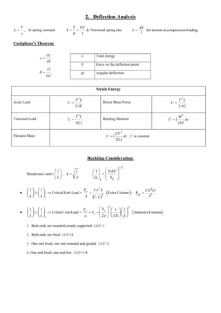
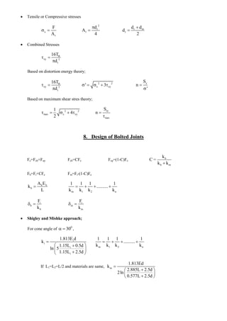
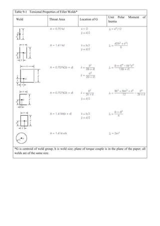
![Table A3-8 Stress concentration factors for round shaft with
shoulder fillet in tension
d
r
D
.
o= F/A, where A= d2/4
D/d =1,02 D/d =1,05 D/d =1,1 D/d=1,5
r/d Kt Kt Kt Kt
0,025 1,800 - - -
0,028 1,728 - 2,200 -
0,031 1,678 2,000 2,125 -
0,037 1,610 1,868 2,020 -
0,044 1,550 1,778 1,938 2,522
0,050 1,508 1,714 1,866 2,400
0,062 1,452 1,626 1,766 2,235
0,075 1,408 1,550 1,684 2,086
0,088 1,370 1,502 1,624 1,970
0,100 1,336 1,457 1,568 1,893
0,125 1,286 1,400 1,496 1,760
0,150 1,254 1,364 1,452 1,662
0,175 1,230 1,340 1,400 1,600
0,200 1,220 1,314 1,372 1,546
0,250 1,216 1,292 1,342 1,508
0,275 1,200 1,270 1,325 1,480
0,300 1,200 1,250 1,296 1,452
* Adopted from Ref. [12]](https://image.slidesharecdn.com/me307machineelementsformulasheet-141102103232-conversion-gate02/85/Me307-machine-elements-formula-sheet-Erdi-Karacal-Mechanical-Engineer-University-of-Gaziantep-13-320.jpg)
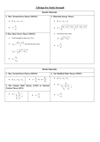
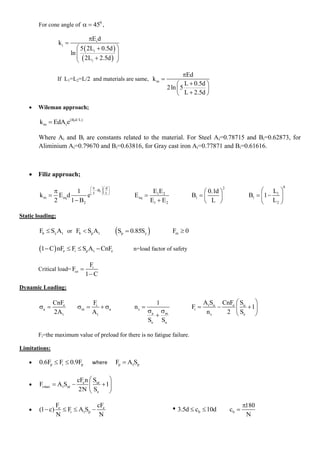
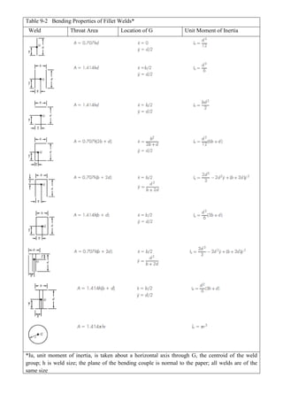
![Table A3-9 Stress concentration factors for round shaft with shoulder fillet
in torsion
d
r
D
T T
.
o= Tc/J, where c=d/2 and J=d4/32
D/d =1,09 D/d =1,20 D/d =1,33 D/d =2,0
r/d Kt Kt Kt Kt
0,009 - - - -
0,012 1,800 2,300 - 2,600
0,030 1,566 2,040 2,144 2,288
0,025 1,472 1,894 2,020 2,122
0,033 1,384 1,761 1,878 1,966
0,042 1,322 1,644 1,755 1,828
0,050 1,283 1,576 1,677 1,750
0,062 1,244 1,500 1,600 1,644
0,075 1,206 1,434 1,516 1,572
0,087 1,184 1,378 1,458 1,510
0,100 1,166 1,342 1,412 1,466
0,125 1,144 1,275 1,344 1,400
0,150 1,122 1,220 1,294 1,344
0,200 1,110 1,160 1,220 1,266
0,250 1,100 1,130 1,178 1,222
0,300 1,100 1,120 1,160 1,200
* Adopted from Ref. [12]](https://image.slidesharecdn.com/me307machineelementsformulasheet-141102103232-conversion-gate02/85/Me307-machine-elements-formula-sheet-Erdi-Karacal-Mechanical-Engineer-University-of-Gaziantep-14-320.jpg)
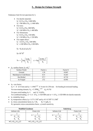
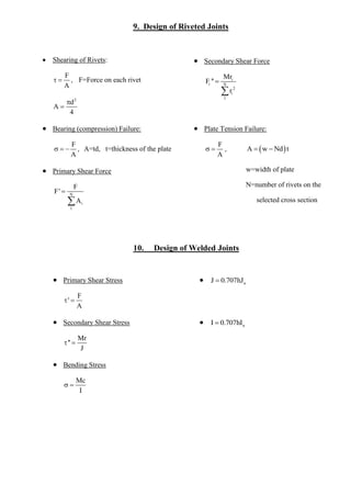
![Table A3-10 Stress Concentration factors for round shaft with shoulder
fillet in bending
d
r
M D M
.
o= Mc/I, where c=d/2 and I=d4/64
D/d =1,02 D/d =1,05 D/d =1,1 D/d =1,5 D/d =3
r/d Kt Kt Kt Kt Kt
0,012 2,290 2,553 2,700 - -
0,017 2,120 2,378 2,500 3,000 -
0,021 2,000 2,240 2,366 2,774 3,000
0,025 1,926 2,134 2,260 2,600 2,862
0,036 1,760 1,936 2,046 2,310 2,600
0,050 1,644 1,782 1,865 2,060 2,310
0,062 1,574 1,700 1,750 1,925 2,140
0,075 1,518 1,628 1,688 1,800 1,986
0,087 1,472 1,563 1,630 1,728 1,880
0,100 1,440 1,534 1,580 1,660 1,804
0,125 1,380 1,468 1,500 1,584 1,684
0,150 1,330 1,412 1,450 1,510 1,584
0,175 1,297 1,358 1,400 1,450 1,510
0,200 1,264 1,336 1,360 1,400 1,457
0,225 1,242 1,308 - - 1,410
0,250 1,225 1,286 - - 1,374
0,275 1,210 1,264 - - 1,340
0,300 1,200 1,242 - - 1,320
* Adopted from Ref. [12]](https://image.slidesharecdn.com/me307machineelementsformulasheet-141102103232-conversion-gate02/85/Me307-machine-elements-formula-sheet-Erdi-Karacal-Mechanical-Engineer-University-of-Gaziantep-15-320.jpg)

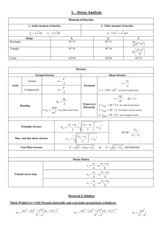
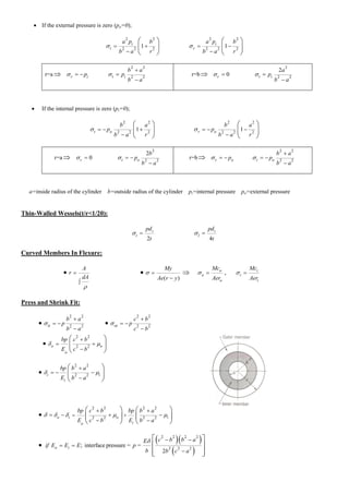
1. The document discusses various topics related to stress analysis including moment of inertias, stresses from different load cases, principal stresses, stress states, stresses in cylinders, and deflection analysis using Castigliano's theorem. 2. Design considerations for static strength are covered for both ductile and brittle materials using theories such as maximum normal stress and distortion energy. 3. Fatigue strength design includes determining the endurance limit based on material properties and adjusting it using factors for surface finish, size, and loading conditions.