SlideShare a Scribd company logo
1 of 244
Download to read offline
1. Earthquake engineering: ground motion, seismic waves, near or
far, foundation design, dynamic seismic soil-structure interaction
(SSI)
1. Sources of Dynamic Loads and Engineering Relevance
5
6
3. Blast and shock engineering: refinery design, homeland
security, defense industry, air and ground shocks, explosion,
mining, ...
2. Wind engineering: high-rises, long bridges, transmission
towers, tall chimneys
7
4. Dynamic foundation design or foundation isolation of
machines/equipment: pump stations, compressors and turbines, high-
tech buildings, wind turbines, …
5. Pile driving & capacity: impact and stress waves, hammer cushions,
bearing capacity determination, NDT, ‘wave equation’ method
6. Impact loading transmitted to foundation and
structures
8
9
7. Offshore foundation engineering
8. Geophysical methods & in-situ sounding
9. Dynamic design for high-speed transportations, tunnels,
buried pipelines
10
10. Construction induced vibrations
….
2. Theory of Dynamics & Vibrations
Basic principles:
• Newton’s laws in physics
• Free-body diagram for dynamic problems
2 types of systems:
• Discrete systems (finite number of degree of freedoms)
• Continuous systems (infinite d.o.f.s)
11
. ., 2 :
nd
e g law m
 
F a m

 i
f a
Discrete systems (finite number of degree of freedoms)
• Lumped mass system:
(a) Single or 1-dof system
12
x(t)
f(t)
(b) Multi-dof system (c) Continuum system
13
14
Analysis of a Single d.o.f. system (SDOF):
(a) sign convention
(b) Free-body diagram (FBD) for
x(t)
f(t)
m
k
c
(c) Write the equation implied by FBD:
( ): ( )
LHS RHS f t k x c x m x
     
   
( )
m x c x k x f t
  
  … a simple 2nd-order differential equation
cx

kx
=
m x

f(t)
m
i
F a


15
1st step: Free Vibration Problem:
Common canonical form of the ‘Equation of Motion’ by
dividing by m,
.... a 2nd-order homogeneous differential equation
0
m x c x k x
  
 
2
2 0 ................ (*)
n n
x x x
 
  
 
.......... ( / )
..........
2
2 2 2 ......
n
n
c n
k
where circular rad s
m
c
m
k
c m m km
m
natural frequency
fraction ofcritical damping / damping ratio
Critical damping constant






 
  
 
 
 
Solution of
Take
• Special case 1: =0 (i.e., undamped case)
16
2
2 0 ......... (*)
n n
x x x
 
  
 
2 2
(*) ( 2 ) 0
t
n n
A e
   
   
2 2
2
1,2
For non-trivial solution, must have ( 2 ) 0
.............. a simple quadratic equation whose 2 roots are
1
n n
n n
   
   
  
   
1,2 1 , , = 1
n n
i i
  
     
( )= ' '
n n
i t i t
x t a e b e
 

 
cos( t) sin( t
s )
cos in n
i t
n
i
n
e i
e i
 
 
 

  
 
Recall
   
( )= ' cos( t)+ sin ( t) ' cos( t)- sin ( t)
( ' ')cos( t) ( ' ')sin ( t)
= cos( t) sin ( t) !
n n n n
n n
n n
x t a i b i
a b i a b
a b
   
 
 

   

( ) t
x t A e

17
( ) cos( ) sin( ) (*)
sin( ) sin cos cos sin .
n n
x t a t b t
trigonometricidentity A A A
 
     
 
  
General solution
:
( ) ( ) 2
2 / ... "natural period"
1/ ... "natural frequency"
( / sec)
2 ... " natural frequency"
( / sec)
/ ....( / sec)
n n n
n n
n n
n n
n
t T t
T
f T
Hz cycle
f circular
rad
with k m rad
  
 
 

  
 
 

 

2 2
(*)... , sin cos , (*)
( )
where " " , " " .
To determine the 2 constants ( , ) or ( , ) in the general solution,
n
n
Taking t a A and b A then is equivalent to
x t A t
a
A a b
b
a b A
   
 


  
 
  
 
-1
= sin( + )
amplitude = phase angle = tan
use initia
0
0
:
(i) initialdisplacement x(0)= x
(II) initialvelocity x(0) = x
l conditions
 
Case (ii) >1 (over-damped case)
18
both are pure exponential decaying terms (no oscillation at all)
2
1,2 1,2
are both -ve from 1
n n
    
   
1 2
( )=
t t
x t a e be
 
 
 
Case (iii) =1 (Critically-damped case)
1 2
= ( . . )
n i e a double root
  
 
   
1
( )= +b +b n t
t
x t a t e a t e

 

 
19
   
2 2
2 2
1 1
1 1
( )= '
' '
n n n n
n n
n n
i t i t
i t i t
t t
x t a e e
a e e b e e
     
   
   
     
  
 

 
Case (iv) 0 <  < 1 (Under-damped case)
- most relevant to geotechnical & structural problems
2 2
1,2 1 1
n n n n
      
       
i
0
0
As in previous cases, can find the 2 constants :
1) initialdisplacement x(0)= x
2) initialvelocity x(0) = x
by initial conditions
 
 
 
 
2 2
1 1
2
= ' '
= ' '
sin ( )
1 ... " "
n n
n
n d d
n
i t i t
t
t i t i t
t
d
d n
e a e b e
e a e b e
e A t
where damped natural frequency
   
 
   
 
 
  
  

 



 
 
20
0 0
Imposing theinitial conditions of
(1) initialdisplacement x(0)= x , (2) initialvelocity x(0) = x ,
one finds
 
Applications: Determination of damping ratio by Logarithmic Decrement method
(for small )
21
1
1
from solution,
n N
n N
t
N
t
N
x Ae
x Ae
Note :
free vibration
zw
zw 






1
1
( )
1
n N
n N N
n N
t
t t
N
t
N
x e
Then e
x e
zw
zw
zw






 
 
 
 
nt
Ae zw

22
ᇱ
ே
ேାଵ
௡ ேାଵ ே ௡ ௗ
ௗ ௗ ௗ ௡
ଶ
ଶ
(II) Forced vibration
23
( )
m x c x k x F t
  
 
2
2 ( ) / ................ (*)
n n
or x x x F t m
 
  
 
0
0
Consider a common and basic form of dynamic load:
................ (*)
.... force magnitude
.... excitation frequency
( ) sin( )
F
F t F t




homog particular
( ) ( ) ( )
x t x t x t
 
General Solution to (*):
( ) ( ) forced vibration
free vibration
or x t x t
 
24
:
sin( ) cos( )
Take A t B t
P f
P
To find x (t) or x (t)
x (t)  
 
 
 
2 2 2 2
0
2 2
0
2 2
2 sin( ) ( 2 )cos( ) ( / )sin( )
/
2
0
2
n n n n
n n
n n
gives
A B A t B A B t F m t
A F m
B
          
   
   
       
 
      
 
     
      
 
2
P n P n P 0
Equation of motion x + 2ςω x +ω x = F / m sin(ωt)
 
2 2
cos( ) sin( )
sin( ) cos( )
then A t B t
then A t B t
P
P
x (t)
x (t)
   
   
 
  


   
 
   
 
2 2
0 2 2
2 2
2 2
2 2
2 2
0
.
/ 2
det / 2
0
/
det / 2
2 0
n
n n
n
n
n n
n
F m
A
F m
B
 
   
 
 
   
 

 
  
 
 
 
 
 
  
 

 
2x2 equations :Solution is (e g. by Cramer's rule)
[ ]
[ ]
25
   
 
     
 
   
 
     
 
2 2
0 2 2
2 2
2 2
2 2 2 2
0
2 2
2 2
2 2
0
2 2
2 2
0
2 .
/ 2
det / 2
0
/ ( ) / 2
/
det / 2
2 0
2 / / 2
n
n n
n
n n n
n
n n
n
n n n
F m
A
F m
F m
B
F m
x2 equations : Solution is (e g. by Cramer's rule)
 
   
 
     
 
   
 
     

 
  
 
 
 
    
 
 
  
 
 
   
 
   
 
   
2
0
2 2
2
0
2 2
2
/ (1 )
1 2
/ 2
1 2
n
F k
A
F k
B
with

 

 





 


 
 
  
 
  where
 
 
 
 

 
   
     
   
     
 
   
 
 
0 n
P 2
2 2
2
n
n n
ω
2ς
F / k ω
x (t) = sin(ωt - ) tan =
ω
ω ω 1 -
1 - + 2ς ω
ω ω
sin( ) cos( )
in A t B t
 
 
P
x (t)
26
 
 
1
( , )
w h ere
S
x



   
   
   
   
 
   
 
 
 
   
   
   
   
 
   
 
 
 

 
0
P 2 2
2
n n
0
2 2
2
n
n n
n
F / k
x (t) = sin (ω t - )
ω ω
1 - + 2 ς
ω ω
D y n a m ic A m p lifica tio n F a cto r Q u a si - S ta tic D eflectio n
ω
A .F . ς F / k
ω
ω ω
1 - + 2 ς
ω ω
ω
2 ς
ω
ta n
f
=
D e in itio n s :

 
 
 
2
n
ω
1 -
ω
: this means the forced response amplitude is
• ( , )
P S
n
Note
x x AF




27
Half-power method for 
using steady-state vibration test data
28
/
1
max
max
and
ark a horizontal line with and find its 2 intesection points
2
with the AF curve and their corresponding frequencies and
1. Identify peak/natural frequency peak amplitude
2. M
peak natural
A
A
w
w
Steps :
2
2 1
.
-
3. Then
2 2
peak peak
w
w w w
V
w w
D

;
36
A simple example of application:
Base isolation design for foundation
0
( ) sin( )
ground motion y t y t


( ) absolute displacement w.r.t. a fixed frame
x t 
Free-body diagram:
=
( )
k x y
 ( )
c x y

 
m x

37
FBDgives the equation: ( ) ( )
k x y c x y mx
    
  
0 0 )
Keeping unknown terms on LHS and prescribed term on RHS,
one gets ( ) sin( ) cos( ) .................(*
mx cx kx k y c y t y k t c y t
  
     
  
   
2 2
0 0 sin( ) ( )
ky c y t F t
  
   
0
Recall the forced response amplitude is
• ( , ), /
P S S
x x AF x F k
 
 
       
   
2 2 2 2
0 0 0 0
2 2
0
max 2 2
2
For (**), .
1 /
Thus
1- 2
p
n n
F ky c y y k c
y c k
x
 

 

 
   


   
   
    
   
 
   
 
 
2
2 2
2
0
1 2
1- 2
2
n
p
Max
n n
crit
x
y
noting c k m



 

 
 
 
  
 
 
 
 
   
   
    
   
 
   
 
 

Ground motion transmissibility
Ground motion transmissibility & design implications:
38
Dynamic Analysis by Complex Notation
39
Recall cos( ) sin( )
i t
e t i t

 
 
 
0 0
2
0
= (cos( ) sin( ))
or 2 .... (*)
/
i t
i t
n n
t i t
x x x
m x c x k x F e F
F m e


 
 

  
  
Consider
 
 
Take ( )=X ei t
x t 

Solution : 2
( )=i X e , ( )= X e !
i t i t
x t x t
 
 
   
 
   
 
0
2 2
0
0
2 2
2
(*)
(
)
( 2
) 2
( 2
)
1
/
n
n
n
n
n
n
t i
hen gives
m
whose solutio
i
X
n is X
i
k
F
F
m
F

   
 

 
   
 
 
 

 
 
 
 

 
   
 
 
   
 
  

 



Note:
1
its form is
a ib

40
0
2
2
2 2
2 2
2 2
:
1/
1 2
1 2
1
1 2 1 2
n n
n n
n n n n
Note
k
X
i
i
k
F
 

 
 

 
   
 
   

 
 
   
 
 
 
   
 
 
   
 
 
 
 
 
 
 
 
 
 
 
 
 
 
   
 
 
   
   
    
       
   
   
   
    
       
   
   
        
   
   
   
 
0
F



41
0 0
2
2
0 0
1
( ) ( ) ( )*
(1 ) 2
( ) is called the function.
Inversely,
(1 ) 2 ( ) (
n n
n n
k
X X F
i
where
k i X or
F or
F F
  
 

 

 
  
 
 
 
 
 
 
 
 
 
 
 
   
 
 
     
 
   
 
 
 
 
 
   
 
 
 
   
 
 
   
 
 
 
C
C Dynamic Compliance
K )
( ) is called the / function
for the model.
X
where  Dynamic Impedance Stiffness
K
i t
F e 
 ( ) i t
x t X e 
 
( )

C
42
0 0
0 0
:
( ) ( ) F sin(ωt) which is the of .
then the corresponding response x(t) must be the Imaginary part of X .
( ) ( ) F cos(ωt), which is the of .
then th
i t
i t
i t
a If F t F e
e
b If F t F e





Results
imaginary part
real part
e corresponding response x(t) must be the Real part of X i t
e 
0
= (cos(ωt)+isin(ωt))as to the equation of moti
a forced excitation of (cos(ωt)+i sin(ωt)), with
i.e., now we got the solution
F
i t
X X
e
0
2
2
0
2 2
2 2
2 2
/
1 2
1 2
1 2 1 2
( ) i t i t
n n
n n
n n n n
k
X e e
i
i
k
F
x t
F
 
 

 
 

 
   
 
   
 
 
 
   
 
 
 
   
 
 
   
 
 

 
 
  
 
 
  
 
 
    
 

   
   
    
       
   
   
   
   
       
   
   
       
   
   
   

(cos(ωt)+i sin(ωt))






 
 

43
2
0
2 2
2 2
2 2
,
1 2
( ) ( * ) sin( ) cos( )
1 2 1 2
i.e
n n
i t
n n n n
x t X e t t
k
F

 

 
 
   
 
   
 
 
 
 
 
 
 
 
 
 
 
 
   
  
 
   
   
   
       
 
   
   
   
   
       
 
   
   
       
   
   
 
   
 
0
For F(t) = sin(ωt)
Im
F
., exactly the same result we had before!
Method of Fundamental Solution (Duhamel integral)
for arbitrary forcing for SDOF
44

f()
t

f(t)
Concept: consider the loading as a sequence of many small impulses.
Tool needed: a Unit-impulse response function g(t,) which gives the
displacement of a dynamic system due to an impulse of unit magnitude at
time  with zero initial conditions.
1
0
We can then write
( ) ( , ) ( )
In the limit of & 0,
( ) ( , ) ( )
N
i
t
x t g t f
N
x t g t f d
  

  

  
   
 


f()
t
45
Next, need g(t,):
: ( ) ( )
.
0 for t except 0
, ( ) 0
( ) 1
.
Solution m x c x k x t or m g c g k g t
with zero initial conditions
at t
In the above the function t at t
t dt
is called the
   




       
 
 
 
 
 
  
 
 
 

 
 

deltafunction
   
t
1/

46
(1) 0 ,
For t 
  0
m g c g k g
  
 
with zero initial conditions
(2) , 0... !
For t m g c g k g free vibration problem also

   
 
( , ) 0
g t 
 
.
o let's use the general free-vibration solution of
( , ) sin( ) .
nt
d
But likely non zero conditions at t after the impulse at time
S
g t A e t for t

 
   


 
  
47
 
+
+
(3) Theimpulse effect going from t= to :
: Consider ( )
Idea m g c g k g t dt


 
 


   
  
+
+
+ +
+
:
1st term: ( , )
2nd term ( , ) 0
3rd term ( ) 0
LHS
m g dt m g m g
m g dt m g m g
m g dt m g dt m g
 


 


 
 
 
 
 






 



 
  
   


 
  

+
:
( ) 1
RHS
t dt


 

 

48
LHS:
1
( , ) 1 ( , )
( , ) 0
m g or g
m
g
   
 
 


 

 
( )
:
0
( , ) 1
sin( ( )
n t
d
d
Summary
for t
g t
e t for t
m
 


  

 

 
 
  
 
 
 
( )
0
giving the solution under arbitrary forcing as
1
( ) sin( ( ) ( )
.
n
t
t
d
d
x t e t f d
m
the
 
   

 
  

Duhamel Integral
1
0
d
A
m

 

Practical Numerical Evaluation of
49
( )
0
1
( ) sin( ( ) ( ) for arbitrary ( )
n
t
t
d
d
x t e t f d f t
m
 
   

 
  

( )
0 0
( ) sin( ( ) sin( )cos( ) cos( )sin( )
( )
sin( ) cos( )
( ) cos( ) ( ) sin( ) ( )
n n n
n n
n n
d d d d d
t t
t t
t t
d d
d d
d d
Note
i t t t
ii e e e
e t e t
x t e f d e f d
m m
    
 
   
       
 
       
 
   
 
 
  

   
 
The two integrals can be numerically by trapezoidal rule or Simpson rule for arbitrary ( ).
f t
Remarks:
1. Good for arbitrary loading
2. Dumhamel integral (a convolution integral)
3. A time-domain method (vs frequency-domain methods)
Numerical Step-by-Step Time Integration Methods
 Direct time-domain procedures
 Allow for nonlinear problems (e.g., a change in k, c, or m as a function
of time and deformation)
 Arbitrary loading time function
 Variety of algorithms and propoals
 Commonly used in FEM, FDM, BEM
 Underlying numerical and discretization issues
50
x(t)
f(t)
m
k
c
f(t)
t
t
51
Idea:
f(t)
t
t
x(t)
t
t
t
x
x
x
 
 
 
 
 

 t+ t
x
x
x 
 
 
 
 
 


forcing
t+2 t
x
x
x 
 
 
 
 
 


forcing
( ) .
m x c x k x f t with some prescribed initial conditions
  
 
t t+t
52
Assumption: the acceleration varies linearly in the time interval of t.

Example : Linear acceleration method :
Writing ( ) , ( ) , ( ) ,
the assumption ( ) 0
t t t
t t t
t
x t x x t x x t x
x x
x t x for t
t
  

  

 
      
 

 
   
 
 
0
2
( ) ( )
2
t
t t t
t t
x t x x t d
x x
x x
t

  

 
 
    
 

    

 

  
 
 
0
2 3
( ) ( )
2 6
0 .
t
t t t
t t t
x t x x t d
x x
x x x
t
for t

  
 



 
   
 

     

 
  
 
 
 

t
x

t t
x 

t t
 
t
53
Taking = t, eq (1),(2), (3) become
 
( ) (1)
t t
x x t t
   
 
( ) (2)
2 2 2
t t t t t t t t t t t
t t t
x x x t x x x x x
  
  
       
       
2 2
(3)
3 6
t t t t t t
t t
x x x t x x

 
 
    
  
i.e., the primary unknown is t t
x 

To find it,
( ) ( ) !
t t t t t t t t
m x c x k x f t at t t m x c x k x f t
   
        
   
54
( )
t t t t t t t t
m x f t c x k x
   
  
 
2 2
( ) ( ) ( )
2 2 3 6
t t t t t t t t t t t
t t t t
f t c x x x k x x t x x
  
   
        
     
2 2
,
[ ] ( ) ( ) ( )
2 6 2 3
t t t t t t t t t
Collecting the terms
t t t t
m c k x f t c x x k x x t x
 
   
        
    
2 2
1
leading to
[ ] ( ) ( ) ( ) (*)
2 6 2 3
t t t t t t t t t
t t t t
x m c k f t c x x k x x t x

 
 
   
        
 
 
    

55
      
1 1
With and computable bymeans of (2) and (3) upon obtaining , one can
collectivelydetermine the displacement, velocityand acceleration at according to
w
[ ] [ ]
t t t t
t t t t t t
t
x x x
t t
 
  
 

 
x f B x
A A
 
   
here
upon defining .
[ ], t t
t
t
x
x
x
and 
 
 
 
 
 
x
B f
A


2
This is a step-by-step algorithm by which
.... !
t t t t t t n t
x x x x
x x x x
x x x x
    
       
       
  
       
       
       
   
   
56
Note:
1) Concept of stability, accuracy, efficiency
a) Conditionally and unconditionally algorithms: a critical time step tcrit
if conditionally stable.
b) Accuracy: Level of numerical amplitude decay/damping & phase shifts
due to accumulation of errors.
c) Explicit and Implicit schemes.
d) Short duration versus long-duration problems.
e) Applicable to MDOF systems (see posted reading)
a) Other methods e.g., Central difference, Newmark method in many
commercial FEM codes (see posted reading)
5
Response Spectrum (a spectral method)
The maximum response of a Single degree of freedom system with
general to a specific excitation (e.g., earthquake ground
motion) :
( , )
n
 
 
2
2 ( )
g
n n g
c x k x m x x
or
x x x x t
 
   
   
  
  
=
-kx-cx m (x+ x )
g
  
( )
g
x t

/
g
x g

6
( )
0
( )
2 0
Analytically, thedisplacement response is expressible in the Duhamel integralform as
1
( ) sin( ( ) ( )
1
sin( ( ) ( ) ..... (*)
1
n
n
t
t
d
d
t
t
d g
n
x t e t f d
m
e t x d
 
 
   

   
 
 
 
  
   


 
max v
pv
( ) ( , ) ....
( , ) ....
d
d
x t S
S
 
 
 Spectral velocity
Spectralpsuedo velocity


 
( )
0
1
( ) ( ) sin( ( ) ( )
n
t
t
d g
d
d
b x t e t x d
dt
 
   

 
   

 
 
( )
pv max
0
( , ) sin( ( ) ( ) is
n
t
t
n d g
S e t x d called
 
     
 
  
 SpectralPsuedo- Velocity

Leibniz rule :
 
0 0
0
( , )
( , ) ( ) ( , ) ( ) ( )
( , )
( )
t t
g g g
t
g
d dt g t
g t x d g t t x t x d
dt dt t
g t
x d
t

    

 

  




 

  

  a
max
(c)
( ) ( ) ( , ) ...
g d
x t x t S  
  Spectralacceleration
 
max
pv
( ) ( ) ( , ) ....
1
( , )
d d
n
n
a x t S
S where
 
 


Maximum response quantities :
Spectral Displacement

7
   
: eqn of motion g
gives m x x c x k x
   
Note   
   max
max
1
g
implies x x c x k x
m
   
  
  2
max
g n d n
k
x x S
m
 
    
d pv
S S
 
Summary of Approximate relations of
Spectral displacement, velocity and acceleration to
Spectral pseudo-velocity
d pv
n
V pv
a n pv
1
S = S
ω
S = S
S = ω S
2
n
n
with
T

 
8
2
2
n
n
T
T




d pv pv
n
V pv
a n pv pv
1
S = S S
ω
S = S
S = ω S S
log log log log(2 )
log log log log(2 )
n
n
T
T


   
   
d pv
a pv
S S
S S
y = m x +b
Line of constant Sd
Line of constant Sa
9
Tripartile plot of response spectrum
10
Design Spectrums
11
Frequency domain analysis
0 0 0
1 0 0
Recall for periodic functions of period T:
2 2
f(t)= sin( ) cos( ), ( )
n n
n n
a n t b n t or T
T
 
  

 
 
  
 
Fourier series
0
0
0
0
0
0
0
0
where
f(t) sin( )
f(t) cos( )
n
n
a n t dt
b n t dt




















0
0 0
0
/
0
/
A much more compact form is
f(t)= = f(t)
2
in t in t
n n
n
F e with F e dt
 
 
 






 
 
0
0 0
0
/
0
/
or
f(t)= = f(t)
2
in t in t
n n
n
F e with F e dt
 
 
 






 
 
t
f(t)
12
0

0
2
0
 0
3
2 2
n n
a b

Can determine the phase angle of magnitude of
each sinusoidal component of f(t)
ie f(t) can be looked upon as a sum of sin( ) !
n n n
A n t
 

Can determine the amplitude/magnitude of each
sinusoidal component of f(t) as 2 2
n n
a b

13
( )= f(t) i t
F e dt







(e.g. an earthquake ground motion or response)
Next : How to treating as non -perioidc function?
0 0 0 0
2
( ) , ( ) / , ( ) , ( ) ( )
n
a d b c n d F F
T

      
      
 
1
f(t)= ( )
2
i t
F e d

 



 
0
1 1
then (*) becomes f(t) ( ) (2)
2 2
in t i t
n
n
F e d F e d
 
  
 
 



 
 

The Fourier transform of f(t) Inverse Fourier transform of ( )
F 

0
0 0
0
/
0 /
Note that
1
f(t)= = f(t) (*)
2
in t in t
n n
n
F e with F e dt
 
 
 






 
 
In the limit of T  
leading to
14

( )
F 

15
Remarks:
 is generally a complex-valued function of
frequency, i.e., with a real and an imaginary part.
 is the Fourier amplitude spectrum (real value)
 Exposes the frequency content of the loading or
response
 It is a full characterization of f(t) in the frequency
domin
 i.e.,
 FFT algorithms (Fast Fourier Tranform)
( ) gives ( ) and ( ) gives back ( ) !
f t F F f t completely
 
 
( )
F 

( )
F 

13
( )= f(t) i t
F e dt







(e.g. an earthquake ground motion or response)
Next : How to treating as non -perioidc function?
0 0 0 0
2
( ) , ( ) / , ( ) , ( ) ( )
n
a d b c n d F F
T

      
      
 
1
f(t)= ( )
2
i t
F e d

 



 
0
1 1
then (*) becomes f(t) ( ) (2)
2 2
in t i t
n
n
F e d F e d
 
  
 
 



 
 

The Fourier transform of f(t) Inverse Fourier transform of ( )
F 

0
0 0
0
/
0 /
Note that
1
f(t)= = f(t) (*)
2
in t in t
n n
n
F e with F e dt
 
 
 






 
 
In the limit of T  
leading to
A Fourier transform pair
14

( )
F 

15
Remarks:
 is generally a complex-valued function of
frequency, i.e., with both real and imaginary parts.
 is the Fourier amplitude spectrum (real value)
 Exposes the frequency content of the loading or
response
 It is a full characterization of f(t) in the frequency
domin
 i.e.,
 FFT algorithms (Fast Fourier Tranform)
( ) gives ( ) and ( ) gives back ( ) !
f t F F f t completely
 
 
( )
F 

( )
F 

16
Basic operational properties:
Fourier transformof derivatives:
[ ( )] ( ) ( )= ( ) w
w
¥
-
-¥
Á = = ò
  i t
recall f t f t F f t e dt
( )
( )
2
( ) [ ( )]= ( ).
[ ( )]
( )
w
w
w w
¥
-
-¥
Á
= Á
=
ò
 


i t
d
b f t f t e dt
dt
i f t
i F
F
( )
( )
( ) [ ( )]= ( )!
w w
Á 
n
n
c f t i F
( )
In integration by part, ( ) ( )
( ) ( )
( ) ( ) 0@
w
w
w w
w
w w
-
¥
-
-¥
¥
¥
- -
-¥ -¥
= -
= +
=  ¥
ò
ò

i t
i t
i t i t
de
f t e f t dt
dt
f t e i f t e dt
i F if f t
( )
) [ ( )]= ( ) ( )= ( ) w w
w
¥ ¥
- -
-¥ -¥
Á = =
ò ò

  
 i t i t
df t
a Consider f t f t F f t e dt e dt
dt
17
:
( )
Solution of SDOF equation of motion under arbitrary forcing
m x c x k x f t
  
Applications :
 
 
To apply Fourier tranform method, consider
( ) i t
m x c x k x f t e dt

  
 
2
( ) ( )
( )
m i c k X F
 
 
 
    
 
 
2
( ) ( ) ( ) ( )
( )
( ) ( )
( ) ( ) .
i t
with
i m X i c X k X F
X x t e dt as the Fourier tranform of x t etc

   

 



   

   

 
( ) i t
m x c x k x f t e dt



  
  
18
2
( ) ( )
1
X F
m i c k
 
 

 
  
  
 
 
or
2
2 ( ) / ................ (*)
n n
x x x f t m
 
  
 
 
2 2
( ) ( )
(*) ( ) 2 /
n n
then gives i X F m
 
   
   
 
 
2 2
2
( )
( )
( )
( ) 2
1
(1 ) 2
n n
n n
m
X
i
k
i
F
F



   
 

 
 
 
 
 
 
 
 
 
 
 
 
  
 
 
   
 
 
     
 
   
 
 
 



19
2
: :
. : 2 ( )
n n g
Example Earthquake ground motion problem
Eq of motion x x x x t
 
   
  
 
 
2 2
/
( ) ( )
( ) ( )
1
( ) 2
n n
x x
X x
i
x
 
 
   
 
 
  
 
 
 
 H 
 



Concept of a Transfer function
Excitation Response
Transfer function
H()
19
2
: Earthquake ground motion problem:
. : 2 ( )
n n g
Recall Eq of motion x x x x t
Example
-
 
  
  
 
 
2 2
/
( ) ( )
( ) ( )
1
( ) 2
g
n n
x x g
X x
i
x
H
 
 
   
 
 
  
 
 
 
 
 



Concept of a Transfer function
Excitation Response
Transfer function
H() of dynamical
system
20

( )
g
x w



( )
X w


( )
w
H
21
Remarks:
 Theoretical modeling characterization of dynamic and
vibratory systems in frequency domain
 Other transfer functions of engineering
interest
/ v/ /
( ), ( ), ( )
. ., g g g
d a a a a
e g H H H
  
 Experimental determination of transfer functions
of physical systems
22

( )
w
H
In more complex systems:
23
2
: (2 )
g n n
a x x x x
Note  
    
  
2
(2 )
n n
a x x
 
   

  
:
: !
g g
g
a x x a x x
Note a x x
Note     
 
 
    
 
  
 
2 2
( ) )
1
( ( )
( ) 2
n n
With X
i
x
 
   
 
 
 
 
 
 
 

 
2
2 2
( )
1
( ) 2
n n
a x
i


   
 

 
   
 
 
 

 
 
 
2
2 2
( )
2
( ) 2
n n
n n
i
a x
i

  
   
 
 

 

 
 
 

 
Re
Im
Z1+ Z2
Z2
Z1
Half-power method for 
using steady-state vibration test data
28
/
1
max
max
and
ark a horizontal line with and find its 2 intesection points
2
with the AF curve and their corresponding frequencies and
1. Identify peak/natural frequency peak amplitude
2. M
peak natural
A
A
w
w
Steps :
2
2 1
.
-
3. Then
2 2
peak peak
w
w w w
V
w w
D

;
Method of Energy Balance
29
 
2 2
1 1
( )
2 2
Kinetic energy m x Potential elastic Energy k x
For a 1DOF :
 
&
x(t)
f(t) A
B
0
( ) sin( ) ( ) sin (
F t F t x t A t for
+ ) undamped free vibration
  
  
 
 
2
2
2
2
Note that KE+PE=
At time A, KE+PE=0 ,
1
2
1
At time B, KE+PE=
2
0
2
1 1
2
n
n n
k A
m A
k
k A m A
m
Conservation of energy
w
w w


 


constant for undamped case
Method of Energy Balance
30
2 / 2 / 2 /
0
Idea: Compare Input nergy & energy dissipated per cycle
( ) sin( ), ( ) sin( ), ( ) cos( )
( ) ( ) sin( )
T T T
input o o o
E
F t F t x t A t x t A t
dx
W F t dx F t dt F t A
dt
p w p w p w
w w f w w f
w w
D
  

    
   
  
Damped 1DOF under Forced Steady State Vibration :
&
 
2 /
0
2 /
2
0 0
cos( )
sin( ) cos( )cos( ) sin( )sin( ))
sin( ) sin ( ) sin( )
T
o
T
o
t dt
F A t t t dt
F A t dt F A
p w
p w
w f
w w w f w f
f w p f



  
 


x(t
) f(t)
 
2 / 2 /
2
2 /
2
( ) ( )
cos( ))
.....
T T
dissip damping
o o
T
o
dx dx
W F t dx t c dt
dt dt
c A t dt
cA
p w p w
p w
w w f
wp
D
 

 
  
 
 
 


 

31
0
2
0
os( )
sin( )
................ (*)
: input dissip
input
dissip
W W
W F Ac
For steady state must ha
W c A
F
A
c
ve
p f
pw
f
w
D D
D
D



 
0
2
max 2
2
/
C a (*) is ident
: ical t
-
o
l
2
im
1
p
n n
F k
x
w w
V
w w

   
   
    
   
 
   
 
 



Hysteretic cyclic stress-strain behavior
in many real materials
32
Area  energy dissipation


Linear viscous model vs physical cyclic stress-
strain behavior :
33
Hysteretic loop’s area’s strong frequency dependency in
linear viscous damper not seen in real materials
x
F
Equivalent Viscous Damping
34
exp
2
exp
2
( ' )
................ (*)
erim
dissip
erim
W c A W hyster loop s area
W
and define
ak
A
T e
equiv
Idea
c
:
pw
pw
D D
D
 

2 2
exp
2
2
(2 )
(2 )
2
equiv equiv
erim crit
crit crit
equiv n
n
equiv
n
c c
W
c
Ta A c A km
c
A km
A
ke
k
Minor - arrangement :
pw pw
w
z p w
w
w
p z
w
D  

 
  
 
exp
2
!
1
4
2
erim
equiv
n
W
kA
z
w
p
w
D
 
   
   
 
 
2
exp
1
4
2
erim equiv
n
W kA
w
pz
w
D
   
    
 
 
• If experimental measurement is done at
35
exp exp
2
!
1 4
4
2
erim erim
equiv
W W
Triangular Area
kA
z
p
p
D D
 
 
 
 
n
 



A
Dynamic Soil Properties
Shear Modulus and Damping:
Stress‐strain response is hysteretic and strain level dependent
Basic engineering parameters:
‐secant modulus G
‐equivalent viscous damping 
both of which are dependent on level of confinement/stress state
2
1
4
2
loop
equiv
G
Area
G



 


 
 
 
• Soil is a particulate/porous
medium
• Under a water table, void
space in the ‘soil skeleton, is
filled by water with pore
water pressure u
SOLID GRAINS
WATER
Importance of effective stresses:
They control:
(a) Shear strength/failure condition in soil
(b) Stiffness/deformability/settlement of foundations
v v
vertical soil effective stress
horizontal soil effective stress h h
u
u
 
 
  
  
v
h



Concept of Effective Stress in Soil
u
In 3D:
Note: Sign convention in soil mechanics:
Compressive stress is positive
Field Measurement Methods:
(I) For low  level (<10‐6 to 10‐4 ) ….. Gmax
(II) Geophysical/wave‐based methods (downhole, cross hole seismic
measurements)
(III) Impulse or low‐level vibration methods
(IV) Shear wave speed: Compressional P‐wave speed:
2 1
1 2
p
G
V

 

 
  

 
s
G
V


Typical range of Vs:
200’/s to 1500’/s for unconsolidated soil.
2000’/s for stiff soils
3000’/s for sandstone
>6000’/s for rocks
E.g., =100 lb/s, Vs=300/s:
Gmax =(100/32.2)(300)^2 = 0.28x10⁶ lb/sqft(psf)
Gmax =(100/32.2)(1500)^2 = 7x10⁶ lb/sqft(psf)
1psf=47.85Pa
1 psi=6.891 kPa
DIFFERENT LABORATORY TESTS FOR DIFFERENT STRAIN LEVELS
Laboratory methods:
Resonant column tests:
‐excited torsionally (or axially) at the top or base
into resonant modes
‐transducers used to measure motion’s time
histories
‐sinusoidal or random excitation
‐use of solid or hollow samples
‐ Equiv viscous damping ratio from hysteretic loop
(r)
Lab tests for higher strain level:
(a) Cyclic simple shear test
Can be stress‐control or strain‐controlled
Drained or undrained (pore pressure development)
Simple shear (stack rings) vs direct shear test
cyclic
h0

cyclic

v0
(v0 ,‐cyclic)
(h0 ,cyclic)
(b) Cyclic triaxial test:
Repetitive axial compression/extension ‐ different stress path
stress control or strain controlled
Drained or undrained (pore pressure development)
0

0+d‐cyclic

d‐cyclic
(0 ,0)
, ,
2(1 )
E
E G G
   

  

~ 0.15 to 0.35 (sand)
0.5 (saturated clay)


(c) Bender element test
Piezoelectric sensors (transmitter and receiver)
Measure average wave speed between 2 points in specimens
s measured
L G
V
t 

 

+ ‐
(d) Shake Table Test
others….
Experimental Synthesis and empirical relationships:
 Gives trends with respect to basic factors
 Different functional forms proposed
 Useful for preliminary assessments
Primary factors affecting shear modulus & damping ratio
Strain amplitude
Mean effective stress
Void ratio
Relative density Dr (sand)
Secondary factors
# of cycles, OCR,  & c, grain characteristics, soil fabric &
structure, frequency, degree of saturation, cementation
Empirical relationships on shear modulus:
 Useful for preliminary assessments
 Gives trends with respect to basic factors
 
 
1/2
2
max 1/2
2
. ., (1972)
(2.973 )
1230 ... angular grains
1 1
( ) ( ~ )
(2.17 )
2630 ... round grains
1 1
0 0
20 .18
40 .30
60 .41
k mean
k mean
e g
e
OCR
e psi
G psi
e
OCR
e psi
PI k
where
-4
Hardin & Drnevich
10



 

 

 
 

 
 
  

 
 

 
 
  
 







 
 
 
 

units of G and p = kg/cm2
Iwasaki et al. (1978)
1/ 2
2
4
2
0..44
2
2 5
max 2
0..4
2
6
2
(1978)
(2.17 )
700 , @10
1 1 /
(2.17 )
( / ) 850 , @10
1 1 /
(2.17 )
900 , @10
1 1 /
mean
mean
mean
e
e kg cm
e
G kg cm for sand
e kg cm
e
e kg cm









 

 

 
 

 
 
 

 

 
  
 
  
 
 

 

 
 
 
  
 
Iwasaki et al
Seed and Idriss (1970)
Separate sand and clay
     
 
1/ 2
max 2 2
max max
2
max
( ) 1000 , 15 0.6 ,
1
0.6 , 2 ,....
( / ) ( , )
mean
u
G psf K K Dr F
psf
F for silt F for gravel
G
kg cm f OCR PI
S
Sand :
Clay :
 
 
  
 
 
 

𝐾
Strain dependence of cyclic shear modulus
• Basic observations: (a) γ
τ
γ
m
m c
g
g
t
= +
max
( ) ,
i As g t t
 ¥ 
m c
g
t
g
 =
+
max
1
m
t
 =
max
0
( ) 0,
d
i As G
d g
t
g
g =
 
( )
2
1
d m
d m c m c
t g
g g g
æ ö
æ ö ÷
ç
÷
ç ÷
ç
÷
 = - ÷
ç ç
÷ ÷
ç ÷
ç ç
+ ÷
è ø ç +
è ø
max
0
1
d
G
d c
g
t
g =
 = =
1 1
1
( ) ( )
max max
max max max
G G
G G G
g
g
g t g t
= +  = +
Summary :
( ) 1 1
1
1
max
ref
max
max max
ref
max
G
where
G
G G
t
g
g
g g
g
t
 = = =
+
+
1
( )
0
max
G
G
g
g


(v ,ult)
(K0v ,‐ult)
cyclic
 c’
max/ult
v
K0v

Basic observation: (b)
1
(i) reverse slope Gmax
(ii) half area of loop constant% * triangle a_b_c’s area
triangle abc’s area
k
»
»
= 
max
1
triangle abc’s area= (ad)(cd-cb)
2
where ad =2
2 /
2 /
cd G
bd G
t
t
t
⋅
=
=
2
1 1
max max
1 1 1 1
area of hyeteretic loop= (2 )2 = 4
k k
G G G G
t t t
æ ö æ ö
÷ ÷
ç ç
÷ ÷
 ⋅ - -
ç ç
÷ ÷
ç ç
÷ ÷
ç ç
è ø è ø
2
1
1
max
2
max
max
max
1 1
4
2 ( )
= 1
1
4 (
2
( )
1
k
k
G G G
Equivalent damping ratio
G
G
G
G
t
g
t p
p
g
z z
æ ö
÷
ç ÷
-
ç ÷
ç æ ö
÷
ç
è ø ÷
ç ÷
= -
ç ÷
ç ÷
ç
è ø
æ ö
÷
ç ÷
 = -
ç ÷
ç ÷
ç
è ø
g
1
( )
0
max
G
G
g
1
0
( )
max
z g
z
Concept of Strain‐compatible shear modulus and damping
To recognize the significant strain‐dependence of the shear modulus and damping ratio,
one generally needs to use a pair of G and  in the dynamic analysis of the model so that
their values are consistent with the strain/deformation level of the response.
Approach:
1. Assume an initial estimate of strain, say, 0 & obtain G(0)
and  (0).
2. Perform dynamic analysis to find the predicted strain level,
say, 1.
3. Check if 1 ‐ 0 is close enough.
4. If not, replace 0 by 1 and repeat step 1 to 4
until difference of the different n+1 and n is
acceptable
5. Then G( n+1) and  (n+1) are called the
Strain‐compatible shear modulus and damping ratio.
* The iterative approach is built in the program SHAKE 91,
2000 for 1‐D equivalent linear ground response analysis
1
( )
0
max
G
G
g
1
0
( )
max
z g
z
0
Multi‐Degree of Freedom Systems
 Soil layering and profile variation
 Improve accuracy and lower degree of
approximation
 Higher‐order wave motion at high
frequencies
Multi-D-O-F system  Continuum system
2
m1
f1(t)
x2(t)
f2(t)
H/2
H/2
, G
, 2G
FBD for Equations of motion for undamped case:
x1(t)
k1
k2
1 1
m x

f1 = 1 1 1 1 2 1
( )
m x k x f
x
 + - =

1 1 2
( )
k x x
-
2 2 1 1 2 2 2 2
2 2 1 1 1 2 2 2
( )
( )
m x k x x k x
or m x k x k x
f
f
k
 + =
+
- -
- + =


f2
2 2
k x 2 2
m x

=
FBD for Equations of motion for undamped case:
1 1 1 1 2 1 (1)
( )
m x k f
x x
+ - =

2 2 1 1 1 2 2 2
( ) (2)
m x k x k k x f
- =
+
+

{ } { } { }
In matrix form  [M] x + f
=
[K] x

{ } { }
1 1
2 2
For the 2-DOF model of the soil layer,
0
....
0
....
3
, ....
m
Mass matrix
m
k k
Stiffness matrix
k k
x f
forcing vector
x f
é ù
ê ú
=
ê ú
ë û
é ù
-
ê ú
=
ê ú
-
ë û
ì ü ì ü
ï ï ï ï
ï ï ï ï
= =
í ý í ý
ï ï ï ï
ï ï ï ï
î þ î þ
[M]
[K]
x f
Note:
M and K are symmetric
{ } { } { } { }
For a damped system, the equation of motion is
+
[M] x [C] x +[K] x f
=
 
{ } { } { }
Case 1: Free vibration of undamped MDOF:
+
[M] x [ 0
=
K] x

{ } { }
{ } { }
) (0)
) (0)
subject to
a
b
=
=
Initial Conditions :
x x
x x
 
Note: Same matrix equation of motion from finite element
methods
{ } { }
As in SDOF:
!
i t
e w
I
=
dea :
x η
{ } { } { } [ ]{ } { }
[ ]
{ }
[ ]
2
2
where the matrix
For non-trivial solution of , must have
det 0.
or
one
w
w
 - + =
é ù
= - +
ê ú
ë û
=
)
=
[M] η [K] η 0 H(ω η 0
H(ω) [M] [K]
η
H(ω)
[ ]
[ ]
2
2
2
2 2 2
0
For the 2-dof example,
0 3 3
with the determinant det ( )( 3 )
m k k m k k
m k k k m k
m k m k k
w
w
w
w w
é ù
é ù é ù
- - + -
ê ú
ê ú ê ú
=- + =
ê ú
ê ú ê ú
- - - +
ë û ë û ë û
= - + - + -
H(ω)
H(ω)
[ ]
( )
( )
2
4 2 2
2
1
2
2
Settingdet 0 4 2 0, a quadratic equation in .
: (2 2) 0.585
(2 2) 3.414
Theyare the of t
k k
m m
k k
Roots
m m
k k
m m
w w w
w
w
æ ö æ ö
÷ ÷
ç ç
=  - + =
÷ ÷
ç ç
÷ ÷
ç ç
è ø è ø
æ ö æ ö
÷ ÷
ç ç
= - =
÷ ÷
ç ç
÷ ÷
ç ç
è ø è ø
æ ö æ ö
÷ ÷
ç ç
= + =
÷ ÷
ç ç
÷ ÷
ç ç
è ø è ø
H(ω)
naturalfrequencies
1
he MDOFsystem.
Put in ascending order, the lowest frequency, i.e., is called the Fundamental natural frequency.
w
Modal shapes associated with each natural frequency
{ } { } { }
( )
( )
{ } ( )
2 1
1 1
1
2
: ... (*) will allow non-unique solutions
2 , (*)
1 2 1 1 2
0
normalize it in
0
1 1 2 1
For a
For the dof system can be reduced to
or
w w
h
h
é ù
- +
ê ú
ë û
é ù ì ü
- + - ï ï
ì ü ì ü +
ê úï ï ï ï ï ï
ï ï ï ï ï ï
ê ú =  =
í ý í ý í ý
ï ï ï ï ï ï
ê ú ï ï
- + î þ
ï ï ï ï
î þ ï ï
ê ú î þ
ë û
1
1
1
[M] [K] η = 0 η
η
{ } { } { }
( )
( )
{ } ( )
2 2
2 2
1
2
different ways
: will allow non-unique solution
1 2 1 1 2
0
0
1 1 2 1
For a
w w
h
h
é ù
- +
ê ú
ë û
é ù ì ü
- + - ï ï
ì ü ì ü -
ê úï ï ï ï ï ï
ï ï ï ï ï ï
ê ú
 =  =
í ý í ý í ý
ï ï ï ï ï ï
ê ú ï ï
- + î þ
ï ï ï ï
î þ ï ï
ê ú î þ
ë û
1
2
1
[M] [K] =
η 0 η
η
{ } { } { }
{ } { } { }
{ } { } { } { } { } { }
{ } { } { } { } { } { }
2
2
2
2
..... (1)
..... (2)
0 ..... (1)
..... (2)
But since the matirx
i i
i
j j
j
T T T
j i j i j
i
T T T
i j i j i
j
and
is also true
w
w
w
w
- + =
- + =
- + = =
- + =
Orthogonality of Mode Shapes
Note : [M] η [K] η 0
[M] η [K] η 0
Observation :
η [M] η η [K] η η 0
η [M] η η [K] η η 0
[K]
{ } { } { } { } { } { }
( ){ } { }
{ } { }
{ } { }
2 2
!
( , too) is symmetic, it is always true that
.
,
(1) (2)
0
0
, !
0
T
j i
i j
T
j
j i
i j
T i
j i
f
and
Ta
i
k
f
i g
i
n w w
w w
w w
-  =
= ¹
=
-
 ¹

T T
T T
[M]
a [K] b = b [K] a a [M] b = b [M]
η
η [M] η
η [K]
a
[M] η
η
{ } { }
We say that the mode shape
with respect the the mass matrix and the stiffness matrix .
i j
is orthogon
]
al
η η
[M
t
[K]
o
Usefulness:
If we put the mode shape vectors in a matrix form
{ } { } { }
{ } { }
{ } { }
1 2
... N
T
T
i i
ii
T
T
i i
ii
then must be
with the diagonal element
must be
with the diagonal element
é ù
= ê ú
ë û
 =
L =
=
Q =
[T] η η η
[T] [K][T] [Λ] a diagonal matrix
η [K] η
[T] [M][T] [Θ] a diagonal matrix
η [M] η
. . diagonalizes both the !
i e and matrices
[T] [K] [M]
0
&
0 3
1 2 1
1 2 1 2
,
1 1 1 2 1
m k k
m k k
é ù é ù
-
ê ú ê ú
= =
ê ú ê ú
-
ë û ë û
é ù
é ù +
+ - ê ú
ê ú
= = ê ú
ê ú
-
ê ú
ë û ë û
T
E.g. For the 2- DOF example of the 2- layered soil,
[M] [K]
[T] [T]
( )
( )
1 2 1 1 0 1 2 1 2
0 1 1 1
1 2 1
T
m
é ù
é ù ê ú
é ù
é ù
+ + -
ê ú ê ú
ê ú
ê ú
= = =
ê ú ê ú
ê ú
ê ú
-
ê ú ë û ê ú
ë û
ë û ê ú
ë û
2
2
1+ 2 +1 0
[T] [M][T] m [Θ]
0 1- 2 +1
1 2 1 1 1 1 2 1 2
[ [ ]
1 3 1 1
1 2 1
T
k
é ù é ù
é ù é ù
+ - + -
ê ú ê ú
ê ú ê ú
= = =
ê ú ê ú
ê ú ê ú
-
-
ê ú ë û ë û
ë û
ë û
4 0
T] [K][T] k Λ
0 4
Modal Analysis of MDOF:
Observation and Ideas:
(i) If the mode shapes are orthogonal to each other. If so, they must be
independent of each other!
(ii) That means any x can be decomposed into a linear combination of
the mode shapes , 1, 2 ...,
i
i N
=
η
{ } { } { } { }
{ }
1 2
1 2
1
2
1
. . ( ) ( ) ( ) ... ( )
( )
..
N
N
N
i
i
i
N
i e t q t q t q t
q
q
q t
q
=
= + + +
ì ü
ï ï
ï ï
ï ï
ï ï
ï ï
ï ï
é ù
= = í ý
ê ú
ë ûï ï
ï ï
ï ï
ï ï
ï ï
ï ï
î þ
å 1 2 N
x η η η
η η η ... η
{ } { }
( ) ( )
t t
=
i.e. let'swrite x [T] q
The s are called the 'Principal' or 'Normal' coordinates of the dynamical system
i
q
With , the equation of motion
{ } { }
( ) ( )
t t
=
x [T] q
{ } { } { } for free vibration of undamped MDOF becomes
+
[M] x [K] x = 0

( )
t
 +
[M][T]q [K] =
[T]q 0

( ) ... (*)
t +
T T
[T] [M][T]q [T] [K] =
[T]q 0

( )
( ) ( )
( )
( )
( ) ( )
( )
1 1 1 1
2 2 2 2
4
4 0 0
4
4 0 0
k
m q k q q q
m
k
m q k q q q
m
+ =  + =
- + =  + =
-
2
2
2
2
1+ 2 +1
1+ 2 +1
1 2 +1
1 2 +1
 
 
1 1
1 1
0.5858 0
3.414 0
k
q q
m
k
q q
m
æ ö
÷
ç
 + =
÷
ç ÷
ç
è ø
æ ö
÷
ç
 + =
÷
ç ÷
ç
è ø


( ) 0!
t + =
 [Θ] q [Λ]q

[ ]
T
Now multiply it by T
( )
( )
& [ [ ]!
T T
é ù
ê ú é ù
ê ú ê ú
= = = =
ê ú ê ú
ë û
ê ú
ê ú
ë û
2
2
1+ 2 +1 0 4 0
Recall [T] [M][T] m [Θ] T] [K][T] k Λ
0 4
0 1- 2 +1
2
1 1 1 1
2
2 2 2 2
0, . . ( )
0, . . ( )
. ., ... (*)
q q i e a SDOF for
i
q t
q q i e a SDOF for q
e gives
t
w
w
+ =
+ =


2
1 1 1
2
2 2 2
( ) ( ) 0
( ) ( ) 0
q t q t
q t q t
of
w
w
+ =
+ =
Solution


i i
A and B
To find the constants , need Initial Conditions :
{ } { } { } { }
{ } { }
( ) ( ) (0) (0)
(0) (0)
t t
=  =
=
Note x [T] q x [T] q
x [T] q


{ } { }
{ } { }
1
1
(0) (0)
(0) (0) !
-
-
=
=
q [T] x
q [T] x
 

1 1 1 1 1
2 2 2 2 2
( ) cos( ) sin( )
( ) cos( ) sin( )
q t A t B t
q t A t B t
w w
w w
= +
= +

Forced Vibration of Undamped MDOF
{ } { } { }
: (t)
Equation of motion [M] x + [K] x f
=

{ } { }
( ) ( )
Take t t
=
Idea : x [T] q
( )
t n t
he +
[M][T]q [ [ =
K T]q f
]

( )
t
T T T
then [T] [M][T]q + [T] [K][T]q [T
= f
]

( )
t
T
then [Θ]q + [Λ]q [T]
= f

1 1
( )
t
- - T
then q + [Θ] [Λ]q [Θ] [T]
= f

1 2
1
is diagonal with diagonal eleme t
(
n s !
is called th
)
e
i
where
t
w
-
-

=
= T
q + [Ω]q [P]
[Ω] [Θ] [Λ]
[P] [Θ] [T] Participation factor matrix
= f

and each is called a
ij
P Participation factor
Meaning of Pij :
Pij gives an indication of how the forcing at the j th mass or node
contribute to the vibration of the ith mode.
1
th
2
e.g., For the i mode's coefficient ,
( ) ( ( )
)
N
i
i i i i j i
j
j
q
q t q P f t F t
w
=
+ =
= å

1 1 2 2 3 3
( ( ( . (
) ) ) )
..
i i i iN N
P f t P f t P f t P f t
= + + + +
{ } { } { } { }
{ }
{ } { }
1 2
1 2
1
1
2
2
With ( ) ( ) ( ) ... ( )
one should note the entire product ( ) represents the 1st mode' contribution,
( ) represents the 2nd mode' contribution, etc to ( )
because the
N
N
t q t q t q t
that q t
q t t
= + + +
ATTENTION :
x η η η
η
η x
{ }
size of depends the chosen normalization of .
i
i
q η
Damped MDOF system under Forced Vibration
{ } { } { } { }
The equation of motion is
+
[M] x [C] x +[K] x f
=
 
:
Solution by modal analysis
{ }
{ } { }
1 2 2
1. Find ... from solving the eigenvalue poblem of [ ]
2. Take ( ) ( )
3. Get [ ... (*)
[
n
t t
w
é ù
= - +
ê ú
ë û
=
+ +
 + +
T T T T
T T
[T] η η η M K η 0
x [T] q
[T] [M][T]q T] [C][T]q [T] [K][T]q [T] f
[Θ]q T] [C][T]q [Λ]q [T] f
=
=
=


1 1 1
[
- - -
 + +
T T
q [Θ] T] [C][T]q [Θ] [Λ] f
=
q [Θ] [T]

[ ] [ ]
[ ] [ ] [ ]
1
1
0
( ) ..... (*)
( ) ( ) ..... (**)
N
j
j
a
b
a b
-
-
=
= +
= å
Particulardamping forms that work :
[C] M K Rayleigh Damping
[C] M M K Caughey damping
1 1
1
4.
2
Will be diagonal generally? If Yes, can write it as 2
and treat the MDOF as N number of SDOF systems, i.e.,
[ i i
etc
z w
z w
-
é ù
ê ú
ê ú
ê ú
ê ú
ë û
T
T] [C][T]
Key Question :
[Θ]
But the Answer is NO generally.
2
1
2 , 1,2,...,
N
i i i i i i ij j
j
q q q P f i N
z w w
=
+ + = =
å
 
[ ] [ ]
, a b
= +
For Rayleigh Damping [C] M K
[ ]
[ ]
1 1
[ [ [
[ [
then
a
a a
a a
- -
- =
 = =
= =
T T
T
Case 1: Mass proportionaldamping [C] M
T] [C][T] T] M [T] Θ]
[Θ] T] [C][T] [Θ] Θ] [I]
[ ]
[ ]
1 1
[ [ [
[ [ ....(**)
then
b
b b
b b
- -
- =
 = =
= =
T T
T
Case 2 : Stiffness proportionaldamping[C] K
T] [C][T] T] K [T] Λ]
[Θ] T] [C][T] [Θ] Λ] [Ω]
Equating to the diagonal matrix of 2 ,
2
2
i i
i i i
i
a z w
a
a z w z
w
 =  =
[I]
2
Equating to the diagonal matrix of 2 ,
one gets 2
2
i i
i
i i i i
b z w
bw
b w z w z
=  =
[Ω]
[ ]
[ ]
2 2
i
i
i
a b
bw
a
z
w
= +
= +
Rayleigh damping Case with [C] M K gives
Modal damping ratio
Note the difference in frequency dependency
[ ]
[ ]
[ ]
[ ] 1
1 2 ...
)
is the
(
N
i i i ij j
j
N
o
wher
r
q q q P
e
f
=
ààà
+ + =
=
å
-1 1
T T
i i i i
T T
i i i i
T - T
[P] = [Θ] [T] [Θ] [ ] Partcipation Factor matrix
η C η η K η
η M η η M η
η η η
 
[ ]
[ ]
[ ]
[ ] [ ]
( )
)
1,2,.., (
i i i
q q q i N
e à
+ àà
+ = =
T T T
i i i i i
T T T
i i i i i i
η C η η K η η f
η M η
N
η M η η M
ot that can also be written as
η
 
1 1 1
[ ( )
- - -
+ + à
T T
q [Θ] T] [C][T]q [Θ] [Λ]q [Θ] [T]
= f
 
Modal form of governing equations for MDOF:
23
Importance of Modal Decomposition in dynamic analysis
• One can choose/select only modes that are important to analyze (e.g., the lower modes in earthquake
problems)
• Can use larger time steps in using direct step-by-step integration methods (for stability and accuracy)
• Without the modal reduction analytically, small time steps will be needed as all higher modes esp. for
a complicated numerical model, are automatically included in the integration but high accuracy is
not quaranteed .
• Artificial numerical damping is thus often employed to damped out high frequency componentwsies
24
Particular Example: MDOF structures subject to Earthquake base motion
{ } { } { } { }
Recall the general equation of motion for MDOF is:
+
[M] x [C] x +[K] x f
=
 
{ } { }
( )
a =
Adaptation to earthquake ground motionproblem?
f 0
{ } { } { } { }
1
1
( )
1
1
ground
b x where
ì ü
ï ï
ï ï
ï ï
ï ï
ï ï
=í ý
ï ï
ï ï
ï ï
ï ï
ï ï
î þ
abs
x = x + 1 1
  
{ } { } { } { } { }
MDOF equation of motion for ground motion is
( ) !
ground
x t effectively
+ =
-
[M] x [C] x +[K] x [M] 1 f
=
  
{ } { } { } { }
With the Equation of motion for MDOF due to base ground motion
ground
x
-
+
[M] x [C] x +[K] x [
= M] 1
  
[ ]{ }
[ ]
2
2 ( )
i i i i i i grou
i i
nd
o q q q x t w ere
r h
V w w a a
æ ö
÷
ç ÷
- ç ÷
ç ÷
÷
=
ç
è
+
ø
T
i
T
i i
η M 1
+ =
η M η
  
{ }
2 1
!
then by the modal decomposition via , one gets
2 ( )
i i i ground
x t
V w w -
+ + = =-
T
x = Tq
q [ ]q [ ]q [Θ] [T] f [P]f [P] ]
= [M 1
  
[ ]
can be diagonalized by the modal shape/modal matrix ,
and assuming [C] T
[ ]
[ ]
[ ]
[ ]
[ ]{ }
[ ]
1 1 2
... , then one can w
,
r
1,2,. ,
ite
( ) ..
o
i i i
N
gr und
M
q q q i N
and
x t
-
-
é ù
= =
æ ö
÷
ç ÷
+ + = ç =
û
÷
ê ú
ë
ç ÷
÷
ç
è ø
T T T
i i
T
i i i
T T T
i i i i i
T
T
i
Recall the Participation facto
η
r matrix i
η C η K η η 1
η M η η M η η M
s
[P] [Θ] [T] [T] η η η
η
  

as the “Seismic
participation factor”
[ ]{ }
[ ]
:
i
i
i i w
a
a
æ ö
÷
ç ÷
ç ÷
ç ÷
÷
ç
è ø
=
T
i
T
i i
Variation of
η M
as a function of or
1
η M η
typically becomes smaller and smaller
at larger and larger natural frequencies .
i
i
numerically
a
w
General observation :
Reason why?
Response spectrum method for MDOF:
2
from solving
2 ( ) ( )
is g
by the response s
.
pectrum, the max
r
ive
response of
a
n by (
( )
due to particu
, )
la
n n ground ground
n
x x
t
x x t x t
x
V w w
w V
-
+
d
R
+
the spectral d
a
isplace
l
ment S
ec l
=
   
[ ]{ }
[ ]
2
Now, in a modal decomposition, the modal coefficient of each mode is gove
(
rned by
2 )
i
i i i i i i gr d
i i
oun
q
q q q x t where
V w a a
w
æ ö
÷
ç ÷
- ç ÷
ç ÷
÷
è
+ =
ç ø
T
i
T
i i
η M 1
=
η M η
+
  
max
the maximum c h
an be given b ( , ) for eac mode !
y = i
i i i
i
q q w V
a
 d
S
How about the maximum value of xi ?
{ } { } { } { }
{ }
1 2
1 2
th
1 2
we defined ( ) ( ) ( ) ... ( ) .
1. the max response of the i mode depends also on the normalization of the
2.the maximums ( ), ( ), ... typically occur at different time
Max
N
N
i
i
t q t q t q t
of q t q t
x q
= + + +
£
R x η η η
η
ecall
Note :
max
1 2
1 max 2 max ... . .
N
i i N i
q q i e RHS is generally an over estimation
h h h
+ + + -
A more optimal and commonly used maximum's estimate is by the " rule":
SRSS
max
1 2 2 2 2
1 max 2 max
max ( ) ( ) ... ( )
N
i i i N i
x q q q
h h h
+ + +

Frequency Domain Analysis of MDOFs
2
)
By modal decomposition, it has been shown that each m
2
ode is g
(
overned by
i i i i i i i
q q q x t
V w w a
+ -
+ =
  
 
2 2
2 2
( )
( )
( )
( ) ( ) ,
( ) )
)
2 (
(
2
i i i ground
ground
i i i
i t
i i i
i i
i
i
q q t e dt as the Fourier tran
q
x
form of q t
then i q
i
x




   

  




 





    
 

  
 
 




 


Define the Fourier transform
 
2
/ / 2
( ) ( ( (
) )
2
)
ground ground
i i i
i q r
a g ound
i i
q a
i
o
e
r
x er
i
wh
q H H


  

   

 

 

 
 
 
 

2
( ) ( )
& & ( )
( )
i i i i
q q
i
q i q
 
 
 
 
   
[ ] { } { } { } { }
1 2
1 2
1
( ) ( ) ( ) ( ) ... ( ) ( )
N
N i
N i
i
t t q t q t q t q w
=
= = + + + = å
Recall x T q η η η η
[ ] { } { } { }
1 2
1 2
( ) ( ) ( )( ) ( ) ... ( ) N
N
q t q q
w w w w w
 = = + + +
x T q η η η

   
{ } { } { }
1 1 2 2
/ / /
( ) ( ) ... ( ) ( )
ground ground ground
N N
q a q a q a x
w w w w
é ù
= + + + ⋅
ê ú
ë û
H η H η H η 

{ }
/
1
( ) ( )
ground
N
i i
q a
i
x
w w
=
é ù
ê ú
= ⋅
ê ú
ë û
å H η 

 
/ 2 2
)
(
2
ground
q a
i
i
i i
i
where
i
H
  




 

 

 
 
 
[ ] { } { } { }
1 2
1 2
( ) ( ) ( )( ) ( ) ... ( ) N
N
q t q q
w w w w w
 = = + + +
x T q η η η

   
{ } { } { }
1 1 2 2
/ / /
( ) ( ) ... ( ) ( )
ground ground ground
N N
q a q a q a x
w w w w
é ù
= + + + ⋅
ê ú
ë û
H η H η H η 

{ }
/
1
,
( ) ( ) ( )
ground
N
i i
q a
i
Concisely
x
w w w
=
é ù
ê ú
=
ê ú
ë û
å
x H η 


Recall g g
x in MDOF x
= =  = =
absolute absolute absolute absolute
Absolute Accelerationsin MDOF :
a x x +1 a x x +1
  
      
1
. .
N
j
j
j
Good to expand in terms of
i e a
=
= å
i
1 η
1 η
Idea? Pre-multiply bothside by ?
i T
η M
1
. .
N
i T j
j
j
i e a
=
= å
T
η M1 η Mη

!
i
j i i
same as the seismic participation factor
a =
T
T
η M1
η M η
( )
1 1 1
( ) ( )
g
N N N
i i i
i i g i i g
i i i
x
q x q x
w w
a a
= = =
+ +
 = =
æ ö
÷
ç
= =
÷
ç ÷
ç ÷
è ø
å å å
absolute absolute
a x x +1
η η η
  
   
   
   
2
Recall 2
i i i i i i ground
i
q q q x
V w w a
-
+ + =
  
2 2
2 (2 ) !
i g i i i i i i i i i
i
q x i q q i q
V
a w w w V w w w
 + =- - =- +
 
    
2
2
i g i i i i i
i
q x q q
V w
a w
 + =- -
  
  /
2 2
( ) ( ) ( ) ( )!
Note that solution for all are similar to the1-dof system's solution, i.e.,
1
( ) 2 g
i
g x x g
n n
q
x x x
i
H
   
   
 
 
 
  
 
 
 
 


 
  
 
2
/ / 2
( )
Recallwe had ) ) )
( ( (
2
ground ground
ground
i i i
i q
i
a a
i i
q
q i
i
x w th
H H


 
  

 

 

 

 
 
 

 
( )
2
2
/
2
2 2
2
(2 )( ( ( )
(2 )
)
)
(
)
2
ground
i ground i i i i i
i i i ground
i i i
ground
i
i
i
i
q a
i
i
q x i q q
i x
i
x
i
V w w w
V w w w
V w w w
w w V
w w
w
a
a
w
w
 + =- -
=- +
+ ö
æ ÷
ç ÷
ç ÷
ç ÷
ç ÷
- + ÷
ç ø
=
è
H
 
   




( )
( )
2
2
1
2
1
( )
(2 )
)
(
2
i i i
ground
i
N N
i i
i
i g
i i
i i i
q x
i
i
x
w
V w w w
w w w
w
a
V
a w
= =
+
æ ö
æ ö ÷
ç ÷
ç ÷
÷
ç ç ÷
 = = ÷
ç ç ÷
÷
ç ç ÷
÷
- + ÷
ç ÷
ç è ø ø
+
è
å å
absolute
a η η 

 
  
( )
( )
( )
{ }
1
2
2 2
2
/ 2 2
1 1
( )
(2 )
(
2
(2 )
where
2
is the vector-va
)
ground
N N
i i
o
i i i
ground
i i
i
i i g
i i
N
i
i
i
md f i i i
a a
i i i
i
q x
i
i
i
x
i
w
V w w w
w w V w
V w w
a
w
w w V
a
w
a
w
w
w
= =
=
+
æ ö
æ ö ÷
ç ÷
ç ÷
÷
ç ç ÷
 = = ÷
ç ç ÷
÷
ç ç ÷
÷
- + ÷
ç ÷
ç è ø
è ø
æ ö
÷
ç ÷
ç ÷
ç ÷
ç ÷
- + ÷
ç
è ø
+
+
=
å å
å
absolute
H
a η η
η
 


  
lued transfer function for a MDOF.
( )
{ }
( )
{ }
( )
{ }
2
2
/ 2 2
2 2
1 1 1 2 2 2
2 2 2 2
1
2
1
1
1 2
1 1 2 2 2
(
2
2 )
2
(2 ) (2 )
2
,
2
ground
mdof i i
i
i
i
i
a
i i
i
a
For a DOF as example
i
i
i
i
i
i
a
w
w
V w w
w w V w
V w w w V w w w
w w V w w w V w
a a
w w
=
æ ö
+
÷
ç ÷
ç ÷
ç ÷
ç ÷
- + ÷
ç
è ø
æ ö æ ö
÷ ÷
ç ç
÷ ÷
ç ç
= +
÷ ÷
ç ç
÷ ÷
ç ç
÷ ÷
- + - +
÷ ÷
ç ç
è ø è
+
=
ø
+
å η
η η
H
( )
Typical profiles of transfer functions H
for MDOFsystems in the frequency domain
w
Dynamics of Continuous System
 Lumped‐mass models (SDOF, MDOF) are inherently an
approximation to many physical systems.
 In geotechnical engineering, the soil region supporting a
building or bridge is inherently a continuous (3D) domain.
 In structural and mechanical engineering:
plate/shell/dome structures,…
 In foundation engineering: earth dams, embankments ….
Multi-D-O-F system  Continuum systems
2
3
Consider a soil or solid stratum/layering
in pure horizontal or simple shear motion y(x,t):
=
x
2
2
y
dx in free vibration
t
r


d
t t
+
t
G, ρ
dx H
( )
2
2
( )
y
a Equation of Motion d dx
t
t t t r

 + - =

2
2
...... (1)
y
Dividing by dx
x t
t
r
¶ 
 =
¶ 
( ) :
...... (2)
b Constitutive relation for shear deformation
G
t g
=
( ) :
................ (3)
c Strain displacement relation for shear deformation
y
x
g
-

=

2
2
...... (1) ...... (2)
y
Together with and G
x t
t
r t g
¶ 
= =
¶ 
one gets
2
2
( ) ......... (*)
y y
G
x x t
r
¶ ¶ 
=
¶ ¶ 
For a homogeneous and medium in free vibration,
G r
2 2
2
2 2
........ 1D classical
........
s
s
y y
C
x t
G
with C
r
¶ 
=
¶ 
=
Wave Equation
shear - wave speed
2 2
2 2
, ( )
y G y y
Generally G
x x x t
r
¶ ¶ ¶ 
 + =
¶ ¶ ¶ 
2 2
2 2
( )
g
y y
G y t
x t
r
æ ö
¶ ¶ ÷
ç ÷
 = +
ç ÷
ç ÷
ç
¶ 
è ø

( ) ?
g
y t
Case of Horizontal Earthquake GroundMotion Acceleration 
2 2
2
2 2
:
0
( )
s
g
Summary
y y
C
y t
x t
the equation of motion for free vibration or forced vibration
of a soil layer inhorizontal shear motion
ì
ï
¶ ¶ ï
- = í
ï
¶ ¶ ï
î

0: (0, ) 0 .
: ( , ) 0
At x y t fixed base condition
At x h H t traction free top surface condition
t
= =
= = -
a) Boundary conditions :
2 2
2
2 2
( ) ( : find the basic dynamic characteristics)
Equation of motion: 0
subject to the above boundary conditions
s
I purpose
y y
C
x t
¶ 
- =
¶ 
Free - Vibration Case
0 0
0: ( ,0) ( ) ( ,0) ( )
At t y x y x and y x y x
= = =
b) Initial conditions :
 
Assume steady-state motion
Approach :
2 2 2
2 2 2
2 2 2
2
2
2
Assume steady-state motion, i.e. take ( , ) ( )
( )
0 ( ) 0
0.
i t
s s
s
y x t X x e
y y d X x
C becomes C X x
x t dx
d X
X
dx C
w
w
w
=
¶ 
 - = + =
¶ 
æ ö
÷
ç ÷
 + =
ç ÷
ç ÷
ç
è ø
Approach :
( ) sin cos for some constants A and B.
s s
X x A x B x
C C
w w
æ ö æ ö
÷ ÷
ç ç
÷ ÷
= +
ç ç
÷ ÷
ç ç
÷ ÷
ç ç
è ø è ø
Solution :
Apply Boundary conditions :
( ) @ 0: (0, ) 0 0 sin 0 cos 0 ( ) sin
s s s
i x y t A B B X x A x
C C C
w w w
æ ö æ ö æ ö
÷ ÷ ÷
ç ç ç
÷ ÷ ÷
= =  = + =  =
ç ç ç
÷ ÷ ÷
ç ç ç
÷ ÷ ÷
ç ç ç
è ø è ø è ø
( )@ : ( , ) 0 (0) cos cos 0
s s
X
ii x H H t G G A H H
x C C
w w
t
æ ö
æ ö æ ö
¶ ÷
ç ÷ ÷
ç ç
÷
÷ ÷
= =  = ç  =
ç ç
÷
÷ ÷
ç ç ç
÷
÷ ÷
ç ç
÷
ç
¶ è ø è ø
è ø
cos 0 ...... (*)
Characteristic/Eigen equation .
s
H
C
is the on the frequency
w
w
æ ö
÷
ç ÷=
ç ÷
ç ÷
ç
è ø
3 5 (2 1)
, , ,.. , 1,2,....
2 2 2 2
s
H i
i giving
C
w p p p p
-
= = =
Implication :
(2 1), 1, 2, ....
2
as the naturalfrequencies of the homogeneous soil layer in shear motion
s
i
C
i i
H
p
w = - =
: ( ) sin sin (2 1) ,
2
i
i
s
x x
Mode Shapes X x i
C H
w p
æ ö æ ö
÷
ç ÷
ç
÷
= = -
ç ÷
ç
÷ ÷
ç ç
÷
ç è ø
è ø
1 1
2 1 2
3 1 2
(2 1),
2
as the frequency & ( ) sin ,
2 2
3
3 as the 2 frequency & ( ) sin ,
2
5
5 as the 3 frequency & ( ) sin
2
s
i
s
C
With i it means
H
C x
fundamental natural X x
H H
x
nd natural X x
H
x
rd natural X x
H
p
w
p p
w
p
w w
p
w w
= -
æ ö
÷
ç
= = ÷
ç ÷
ç
è ø
æ ö
÷
ç
= = ÷
ç ÷
ç
è ø
æ ö
ç
= = ç
ç
è
...... for a stratum.
÷
÷
÷
ø
homogeneous
3 6
1 1
1
: 100', 100 / , 0.25 10
283.7 / sec
2
4.457 / sec 1.41sec
s
Example Homogeneous soil layer H g lb t G psi
G
C ft
rad T
r
r
p
w
w
= = = ´
 = =
 =  = =
:
Forced Vibration due to ground motion
1
2
2
1
2
2
1
:
( , ) ( ) ( )
( ) ( )
( ) ( )
i i
i
i i
i
i i
i
Let y x t q t X x
y
q t X x
x
y
q t X x
t
=
=
=
¥
¥
¥
=

¢¢
 =


 =

å
å
å
Modal expansion approach

2 2
0
for all mode shapes
i i
i i i i
s s
X X X X
C C
w w
æ ö æ ö
÷ ÷
ç ç
¢¢ ¢¢
÷ ÷
+ =  =-
ç ç
÷ ÷
ç ç
÷ ÷
ç ç
è ø è ø

2
1
( ) ( )
i
i i
i s
q t X x
C
w
=
¥ æ ö
÷
ç ÷
=- ç ÷
ç ÷
ç
è ø
å
2 2
2
2 2
( )
s g
y y
C y t
x t
¶ 
- = 
¶ 

2
1 1
2
1
( ) ( ) ( ) ( ) ( )
( ) ( ) ( ) ( )
i
i i i i g
i i
s
i
i i i g
i s
q t X x q t X x y t
C
q t q t X x y t
C
w
w
= =
=
¥ ¥
¥
æ ö
÷
ç ÷
- - =
ç ÷
ç ÷
ç
è ø
æ ö
æ ö ÷
ç ÷
ç ÷
ç ÷
 + =-
÷
ç
ç ÷ ÷
ç
ç ÷
ç ÷
è ø ÷
ç
è ø
å å
å
 
 
i j
Orthogonality of X and X :
2
How? From 0
i
i i
s
X X
C
w
æ ö
÷
ç
¢¢ ÷
+ =
ç ÷
ç ÷
ç
è ø
2
0
0
0 0
0 .... (1)
H
i
i i j
s
H H
H
i j i j i j
Consider X X X dx
C
and X X dx X X X X dx
w
æ ö
æ ö ÷
ç ÷
ç ÷
ç ¢¢ ÷
+ =
÷
ç
ç ÷ ÷
ç
ç ÷
ç ÷
è ø ÷
ç
è ø
¢¢ ¢ ¢ ¢
= -
ò
ò ò
2
0
0
0 0
0 ...... (2)
H
i
j j i
s
H H
H
j i j i j i
Likewise X X X dx
C
and X X dx X X X X dx
w
æ ö
æ ö ÷
ç ÷
ç ÷
ç ¢¢ ÷
+ =
÷
ç
ç ÷ ÷
ç
ç ÷
ç ÷
è ø ÷
ç
è ø
¢ ¢ ¢ ¢ ¢
= -
ò
ò ò
0
( ) ( ) 0
H
i j
X x X x dx if i j
= ¹
ò
0
& 0
H
i j
X X
¢ =
2
1
0
2
0 0
( ) ( ) ( ) ( )
( ) !
( ) ( ) ( ) ( ) ( ) ( )
j
j j j g
i s
H
i
H H
i
i i i i g i
s
Then take q t q t X x y t
C
and multipleby X x dx and
q t q t X x X x dx y t X x dx
C
w
w
=
¥ æ ö
æ ö ÷
ç ÷
ç ÷
ç ÷
+ =-
÷
ç
ç ÷ ÷
ç
ç ÷
ç ÷
è ø ÷
ç
è ø
æ ö
æ ö ÷
ç æ ö
÷
ç ÷
ç ÷
ç
÷
 + =-
÷
ç
ç ÷
÷ ç ÷
÷
ç è ø
ç ÷
ç ÷
è ø ÷
ç
è ø
å
ò
ò ò
 
 
2
0
2
0
( )
( ) ( ) ( )
( )
4
( )
(2 1)
H
i
i
i i g H
s
i
i g i
X x dx
q t q t y t
C X x dx
y t where
i
w
a a
p
æ ö
÷
ç ÷
 + =-
ç ÷
ç æ ö
÷
ç
è ø ÷
ç ÷
ç ÷
è ø
=- =
-
ò
ò
 

Damping:
:
: , ...
G or E c
t g V g s e e
= + = +
Theory of Viscoelasticity
Kelvin - Voigt 

k
c
Maxwell :
G
t t
g
V
= +


2
2
( ) Equation ofMotion ...... (1)
y
a
x t
t
r
¶ 
=
¶ 
( ) Constitutive relation for viscoelastic model in shear deformation:
...... (2)
b
G
t g V g
= + 
( ) :
................ (3)
c Strain displacement relation for shear deformation
y
x
g
-

=

2 3 2
2 2 2
(1),(2) (3),
0
......... (*)
( )
g
Combining and the equation of motion with viscous damping is
y y y
G
y t
x x t t
V r
r
ì ü
ï ï
¶ ¶ ¶ ï ï
+ - = í ý
ï ï
¶ ¶ ¶ ¶ ï ï
î þ

: ( , ) ( ) ( )
... modal decomposition
or method of separation of variables in p.d.e.s
Take y x t q t X x
idea of
=
Solution
2 3 2
2 2 2
2
2
(*)
0
( )
0
......... (**)
( )
( ) ( ),
0
( )
g
S
g
S
g
Then leads to
G y y y
y t
x x t t
C q X q X q X
y t
Dividing by T t X x
X q X q
C
y t
X q X q
V
r r
V
r
V
r
ì ü
ï ï
¶ ¶ ¶ ï ï
+ - = í ý
ï ï
¶ ¶ ¶ ¶ ï ï
î þ
ì ü
ï ï
ï ï
¢¢ ¢¢
⋅ + ⋅ - ⋅ = í ý
ï ï
ï ï
î þ
ì ü
ï ï
¢¢ ¢¢ ï ï
+ ⋅ - =í ý
ï ï
ï ï
î þ

 

 

2
2
2
2
2
0 .... ( ) ( :1st term is a function of x only.
constant, say= ....( ),
( ) 0
with the boundary conditions of (0) 0 ( ) 0.
S
S
S
X q X q
C Note
X q X q
X
Taking
X C
then X X
C
X and X H
V
r
w
w
¢¢ ¢¢
+ ⋅ - = 
¢¢
= - 
¢¢
  + =
¢
= =
For free vibration :
 
Recall we found
(2 1) ( ) sin sin (2 1) 1, 2, ....
2 2
for a homogeneous soil layer in shear motion
s i
i i
s
C x x
i and X x i for i
H C H
p w p
w
æ ö æ ö
÷
ç ÷
ç
÷
= - = = - =
ç ÷
ç
÷ ÷
ç ç
÷
ç è ø
è ø
2
2 2
2
2 mode ,
2 2
2 0
.... mode free vibration !
i i i
i i i
S S i
i i i i i
th
Setting which increases with number
C C G
q q q
a damped SDOF equation for i in
w V w V w
V
V w V
r r
V w w
æ ö
÷
ç ÷
=  = =
ç ÷
ç ÷
ç
è ø
 + + =
 
2 2
2 2
2 2
( ),
( ) 0 0 ..... (***)
S S
With
q q
q q q
q q C C
V w V w
w w
r r

æ ö æ ö
÷ ÷
ç ç
÷ ÷
  + ⋅ + =  + + =
ç ç
÷ ÷
ç ç
÷ ÷
ç ç
è ø è ø
 
 
2
,
the governing equation
2 ( ) with the extra damping term
4
with for the homgeneous soil case.
(2 1)
i i i i i j g
i
becomes
q q q y t
i
V w w a
a
p
+ + =-
=
-
For the earthquake ground motion problem
  
(2 1), 1, 2, .... naturalfrequencies
2
s
i
C
i i
H
p
w = - =
( ) sin sin (2 1) , ...
2
i
i
s
x x
X x i mode shapes
C H
w p
æ ö æ ö
÷
ç ÷
ç
÷
= = -
ç ÷
ç
÷ ÷
ç ç
÷
ç è ø
è ø
v
1
max
Recall for a homogeneous layer,
( , ) 4
with (2 1)
(2 1)
i i
i j i i
i
S
q and i
i
w z
a a w w
w p
= = = -
-
:
Example : Modal contribution to response quantities by R
Applications and insights from Ex
esponse Spectrum :
act Solutions
v v
2
max max
1 1
v
2 2
( , ) ( , )
4 4
( , ) ( ) (1)
(2 1) (2 1) (2 1)
4 ( , ) 1 1 1 1
~ 1, , , ...
(2 1) (2 1) 9 25
i i i i
i i i
i i
S S
y H t q X H
i i i
S
where
i i
w z w z
p w pw
w z
pw
æ ö æ ö
æ ö ÷ ÷
÷ç ç
ç ÷ ÷
 = = ÷ =
ç ç
ç ÷ ÷
÷ç ç
ç ÷
ç ÷ ÷
ç ç
- - -
è øè ø è ø
æ öæ ö
÷ ÷
ç ç
÷ ÷ =
ç ç
÷ ÷
ç ç ÷
֍
ç - -
è ø
è ø
1
max a v
Similarly,
4
( , ) ( , ) ( , )
i j i i i i
a H t S S
w
a w z w z
p
= = 1
Note: there are now 2 regimes of dynamic behavior:
depending on whether  is > or < than cutcoff
( )
1 1
( , ) ( ) ( ) ( )
2 2
x ct
x ct
y x t f x c t f x c t g d
c
h h
+
-
= - + + + ò
Basic Wave Propagation Theory
in 3D for Soil Dynamics & Seismology
R. Y. S. Pak
2
Homogeneous & isotropic with 2 elastic constants ( )
1 2
Based on (i) Newton'slaw, (ii) stress-strain relationship & (iii) small strain theory
(Navier's equation):
( 2 )
G
and G
G

 


Equationof motion
- =
-
-
-
+
( )
2
1 2 3
, ,
2
2 2
2
( ) ( )
( ) ( )
In rectangular coordinates with , , ,Navier's equation becomes
( ) ,
( ) , (repeated index
k ki i kk i
i
k i
k i k k
i 1,2,3
i 1,2,3
G
or G G
u u u
G u Gu u
u
u u
G G
x x x x t

 
 
 
u u u
u u u
u
=
=
 ⋅ - ´ ´ =
+  ⋅ +  =
=
+ + =

¶ 
 + + =
¶ ¶ ¶ ¶ 



3
1
2
2 2
3 3
2
1 1
,
)
( )
k
i
k i
k k
k i k k
i 1,2,3
u
u u
G G
x x x x t
 
=
= =
=


¶ 
 + + =
¶ ¶ ¶ ¶ 
å
å å
Formulation for 2D/3D Soil Dynamics and SSI Problems
12
13 11

 
1 1 2 3
2
. ., sin ( ) , 0
d
d
e g u A x C t u u
L

 
   
 
 
• a sinusoidal plane compressional/dilatational or P-wave train of wave length Ld
• a solution of the Navier’s eqn of motion
2 1 1 3
2
. ., sin ( ) , 0
s
S
e g u A x C t u u
L

 
   
 
 
• a sinusoidal plane shear or S-wave train of wave length Ls
• a solution of Navier’s eqn of motion
Examples: Plane waves solutions:
x2
x1
x3
with ... shear wave speed
s
G
C

=
2
with ... compressional/dilatational wave speed
d
G
C


+
=
3 2
1
2 3
1 2 3
3
1
2 3, 2
1 2 3 1 2 3 3 1
1 2 3 2 1
3
1 1
2
x x
where
x x x x x x x x
x x
 


  

    
 
 
 
 
 
 
 


     
        
 
       
 
 
 

 
 
 
1
e
e e e
e e e ψ e
e
subject to boundary, initial and loading conditions
General Solution by Method of Potentials:
Take 
   
u ψ
2 2
2 2
2 2 2 2
2 2 2
2
2 2 2
1 2 3
Then Navier's equation becomes
1 1
, ( ave equations in 3D)
with
d s
w
C t C t
x x x


 
   
 
  
   
  
ψ
ψ
Plane waves propagating in arbitrary 3D directions:
In terms of the 2 potential functions:
( ) ( , ) ( ) ( , ) ( )
. ., is the direction of the unit vector which denotes the direction of wave propagation
with compressional/dilatational wave speed ... i.e. a P-wav
d d
d
a x t f C t x t f C t
ie
C
d d d
d
k x u k k x
u k
  
       
e.
( ) ( , ) ( ) ( , ) ( )
. ., is orthogonal to the unit vector which denotes the direction of wave propagation
with shear wave speed ..... i.e. a S-wave.
The sh
s s
s
b x t C t x t C t
ie
C
s s s
s
ψ g k x u ψ k g k x
u k
Note:

        
ear wave motion can be decomposed into
a Horizontally-polarized (SH) shear wave and a Vertically-polarized (SV) shear wave.
x
Wave propagation direction
SH wave motion (out of plane)
SV wave motion (in‐vertical plane)
z
y
O
x1 or x, u1 or u
x2 or y
u2 or v
x3 or z, u3 or w
2
2
3 2
1
1 2 3
2 1
3
3 1 2
0 ( ):
( )
( )
2
With u and plane strain
x
u u
x x x x z
u w
x x x z x
depend on only scalar potential functions and
 
  
 
  
 



 
  
     
    
 
  
     
    
Simplification for 2D Wave Propagation Problems (Plane Strain):
2 2
2 2
2 2
1 1
,
d s
C t C t
 
 
 
   
 
3 2
1
2 3
1 2 3
3
1
2
1 2 3 3 1
1 2 3 2 1
3
1 1
2
x x
x x x x x
x x
 


    
 
 
 
 
 
 
 


  
    
 
    
 
 
 

 
 
 
e
e e e
ψ e
e
Example: Time harmonic Incident Plane P- and SV-waves
in a Semi-Infinite Soil in 2D (Plane-strain)
n
l
Solution:
sin 2(1 )
where = , the ratio of compressional to shear wave speed
sin (1 2 )
s d d
d s s
C C
k k
C C

 
  

   

Physical phenomena of wave
reflection, mode conversion,
diffraction, refraction,...
1 2
Other important wave types and solutions of boundary value problems of soil dynamics and
seismological interest:
- Rayleigh waves (a surface wave with motion decaying quickly with depth) with wave speed CR (< CS< Cd)
- Theoretical basis of site/soil characterization by wave-based methods and forced vibration testing
(eg dynamic load on finite area)
- Fundamental to seismic/dynamic soil-structure
- Extension and applications to multi-layer soil configurations
Dynamic foundation response from applied loads
(SSI problems)
Incoming SH wave (simpler than SV wave)
with 1 = 2
Dynamic Soil-Structure Interaction
(551) Problems
ExamDle: A Comoressor Foundation Dynamic Problem
Rigid body dynamics: F=ma, M=Icx
Soil
Soil
e at (0 rad/sec
Needed material information:
Establish soil/site/foundation/structure conditions
•Dynamic loading, nature, magnitudes and directions
•Soil profile: sand, clay, rock, thickness, layering,
•Density, void ratio, P1, OCR,
•Dynamic shear modulus G and damping with their strain
dependence
•Machine’s mass, moment of inertia, stiffness
‘Foundation type, shape, weight/bearing pressure
‘Design criteria
Example: Characterization of dynamic loads
Newton’s law: F= m a, M= ‘M
Mmachine
Soil
Resultant
dynamic loads:
F=me rw2 = m7v2/r
5 to 10% rotating mass
= Fsin(wt) or
F = Fsin(at)
F = FcosQot) F, = Fcos(cot)
Fundamental example problem:
A Rigid footing under dynamic loading
• A Mechanics Contact problem
• 3D elastodynamic theory and wave radiation phenomena
• Interface & boundary conditions
• Concept of radiation damping
• Analytical methods
• Finite element and boundary element methods
• Frequency and time domain
I
i-i I foundation
interface
Foundation Interfacial Impedance Matrix
V K(w) 0
H 0 0
M 0 0
T 0 KTT(co) ®
• From solution of 3D continuum boundary value problems
• In frequency domain / time-harmonic factor ebo)t
• Each function is generally complex-valued for nonzero (0
i.e., K1 (w) = Re[K (w)] + i Im[K (w)]
• ‘Dynamic foundation impedance functions’
• Contact stress distributions
• Horizontal-rocking motion coupling
Note:
1. Notion of ‘Frequency
(*)
dependent’ springs and
dashpots due to 3D wave
propagation phenomena
2. Radiation/geometric
damping
i.e. a mechanical analog of Impedance Functions (suggestion by Lysmer 1965)
0
Khh(o)
Kmh (0)
0
0
Khm (t0)
Kn?m (t0)
0
Recalifrom SDOF with spring-rnass-dasphot:
F(t)=kx(t)+c 1(t) F(o)=kx+kocx =‘F(o)=(k+iwc)x=K(w)x ....(*)
Comparing it with
K(co)=Re[K(w)]+ i Im[K(w)]
one can set
k =Re[K1(o)] =k(w)
c= Jm[K(o)]/w=c(o)
= 2 = Ccriticai
Foundation Interfacial Compliance Matrix
C (w) = Re[C (w)] + i Im[C1 (w)]
- //,‘
*I
‘
C(w) 0 0 0 V
Ah — 0 Chh(w) Chm(W) 0 H
Or — 0 CmhfrO) Cmm(CO) 0 M
°T 0 0 0 CTT(a)) T
• jCJ=[K]’
• Symmetric matrices due to reciprocity property in elastodynamics theory
• Depend on foundation shape, type, embedment, soil profile,
• Examples for circular and square surface foundations:
•
Classical Solution for Foundation Compliance Functions by Homogenous Half-space model:
Notation: a=radius, a=Poisson ratio, i=shear modulus (Luco & Westmann (1971)
16
/I
7
.6 -
__zr— ‘
Square foundation impedance functions by Homogenous Half-space model:
(Pak & Guzina 1999)
Rk SlfCsf of Sqs Sfc, F d.ss
Hp El. H,If-S
k =ic =-
‘ Gb’
hh
Gb
K,
k Kmm
mhGb2 mm
Gb3
r
,‘97Ib!fI3
.i
FIg 0-21 V,siI ,ibSi ( dI f,,Sim. f 4
Fry (1963), Richart, Hall & Woods (1970)
Results from centrifuge model tests
*
Pak et al. (2010) “Physical Characteristics of Dynamic Vertical-Horizontal-Rocking
Response of Surface Foundations on Cohesionless Soils,” Geotechnique
G=shear modulus, v=Poisson ratio, b=half-width
V,s1,,j SifY,p cf a Sql,aa Sda,a F,,,,d.,,,
HopSaCC ElsO, HaJf-0p.a
IC =
CpIi,.g Cf• Sq F,.,,d.U,,
H.
LS,aJ OCtl,,aa,, Sqaa 0IISCS PCCIiII
HCgaC E. Hi1-S
soc. 00.6
Results from experimental field tests
sEC. 0.7 R1XKf3JVIHR4rIoS5 30 FOIJ’4DATIONS 371
0
FI0C,a 0-06. CsopIad sskICga,d .1___i__Ji_..._. so1
,IICjC ,ibIoI,,,a ,f WES Ba,a . 8, 337
I. Taos 36. (a) CI5O5Cs,ao ‘t’ B,’C CI
C 0.33 2C
A,,.,,,
Reasons:
1: In-situ depthwise variation ofshear modulus ofreal soils
(i.e., generally not homogeneous)
e.g., sand, gravel, or NC clay
2: Theoretical vs physical contact stress distributions
small-strain theory
(a)
failure limit
(b)
actual service state
(c)
3: Effects of foundation weight and loading
If
Analytic Resolution by New Elastodynamic 551 Theory
(Pak and Ashlock, EESD 2011)
1.5
0 Depth ratio
E hf/b
0 Modulus ratio
,=
—
0.5
Standard elements
AG elements
2
10
y/a xla
R. Y. S. PAK AND J. C ASHLOCK
—1
0 1 2
cøa / (G0/p)°5
(d)
Vertical, Horizontal, Rocking Foundation Responses
—
— .254.0 14. c1.6
-
y45. c3.2 —j4.5. c1.5
‘ 2, 2.4 -:=5. ‘1.3
.
1=3.5)=19 =1 05
0 500 1000 1500
Frequency [Hzl
500 1000 1500 2000
Frequency 1Hz]
3
0
0
E
E
2’:
2
E
Cu
0
0
rn
1 2
wa I (G0/p)°5
Figure I I. Impedance functions K11() by 2-zone theory with h= I. (a) K,,:
(b) Ku,,: (C) K,,,,,: and (dl K,,,,, and Kh,,,.
/ -H
.-
2000
—
— C=.25.n=4.0 — 0=4. ã=1.6
n=2.5. 2=3.2 : C=4.5. 2=1.5
-0=3. G=2.4 —-0=5. 2=1.3
O 0 .)35. =19 .4=0,2=1.0S
- -.
—b
Mechanical Analogs of Impedance Functions for simplified analysis
F(t)=kx(t)+c±(t) F(do)=kx+iacx
=F(o)=(k+iac)x=K(oi)x ....(*)
Comparing it with
K11(o)=Re[K1(w)]+i [m[K1(eo)]
one can set in (*)
k = Re[K. (w)] = k(to) Note:
U 1. Notion of ‘Frequency-dependent’ springs
c = Im[K1 (w)] / tü = c(a) and dampers (3D wave propagation
phenomena
— C — C 2. Concept of Radiation/geometric
1i damping
4J !W1t critical
Use: Convert differential equations of motion
to simpler algebraic equations:
-1
2
( ):
F[ ( )] ( ) ( )
:
1
F [ ( )] ( )
2
:
F[ ( )] ( ) ( ), F[ ( )] ( ) ( ) , .
i t
i t
Fourier transform of a function f t
f t f t e dt
Inverse Fourier transform
e d
Key properties
f t i f t i etc



  

   





 

 


 
F
F F
F F
Frequency‐Domain Approach:
(1) Vertical vibration:
Time harmonic response,
i.e.
( ) , ( ) ,....
i t i t
F t e t e
 
  
F Δ
Frequency‐domain Dynamic Analysis of Foundations
0 vv 0 0 G
V =K (ω)Δ & Δ =Δ
......(1)
v e o
F V m
   

G

2
v-e o G
F -V =-ω mΔ
=
v
m

v

Fv‐e
V0
2
v-e vv G G
F -K (ω)Δ = -ω mΔ
...(2)
v-e
G 2
vv
F
Δ =
-ω m +K (ω)
଴
(a) Equations of Motion:
x x
F m
 
 
(2) Horiz‐rocking coupled vibration:
 
F ma, M I α
G G
M I

 
G
I 

o
H
= G
m

e
F e
M
G
O
1
2
d
d
2b
o
M
o
H
...............(1)
e o G
F H m
   
 2
e o G
F -H =-ω mΔ
1 2 .....(2)
e e o o G
M F d H d M I
    
 2
e e 1 o 2 o G
M +F d +H d -M =-ω I θ
...(3)
     
 
 
     
 
 
   
     
G o e
2
G o e e 1
2
Δ H F
1 0
m 0
-ω + =
θ M M +F d
-d 1
0 I
(b) Foundation‐soil interfacial impedance relations:
.............(4)
    
   
 
    
o hh hm o
o mh mm o
H K K Δ
=
M K K θ
.............(5)
      
 
 
     
 
 
 
   
      
G hh hm o e
2
G mh mm o e e 1
2
Δ K K Δ F
1 0
m 0
-ω + =
θ K K θ M +F d
-d 1
0 I
(c) Relation between motions at different points :
0
G


G
o


o

o

............(6)
   
 
   
 
 
   
o G G 2
o G
o G
2
o G
Δ =Δ -θ *d
θ =θ
Δ Δ
1 -d
=
θ θ
0 1
2
d
(d) Final equation assembly:
Substituting (6) to (5), one gets
2
( ) .............(7)


 
  
 
M K F
x

0
,
0
m
I
 
  
 
M
2
2
1 0 1
1 0 1
hh hm
mh mm
K K d
K K
d

 
   
  
   
  
   
K

1
, ,
G e
G e e
F
M Fd


   
 
   

   
x F
where
The matrix equation (7) for coupled lateral response motion can be readily
solved for any given loading F .
dynamical analysis of soil and structures

More Related Content

Similar to dynamical analysis of soil and structures

Integral calculus formula sheet
Integral calculus formula sheetIntegral calculus formula sheet
Integral calculus formula sheetAjEcuacion
 
Integral calculus formula sheet
Integral calculus formula sheetIntegral calculus formula sheet
Integral calculus formula sheetHimadriBiswas10
 
Circuit Network Analysis - [Chapter4] Laplace Transform
Circuit Network Analysis - [Chapter4] Laplace TransformCircuit Network Analysis - [Chapter4] Laplace Transform
Circuit Network Analysis - [Chapter4] Laplace TransformSimen Li
 
Mcrowave and Radar engineering
Mcrowave and Radar engineeringMcrowave and Radar engineering
Mcrowave and Radar engineeringPriyanka Anni
 
Me307 machine elements formula sheet Erdi Karaçal Mechanical Engineer Univers...
Me307 machine elements formula sheet Erdi Karaçal Mechanical Engineer Univers...Me307 machine elements formula sheet Erdi Karaçal Mechanical Engineer Univers...
Me307 machine elements formula sheet Erdi Karaçal Mechanical Engineer Univers...Erdi Karaçal
 
Engineering Mathematics 2 questions & answers
Engineering Mathematics 2 questions & answersEngineering Mathematics 2 questions & answers
Engineering Mathematics 2 questions & answersMzr Zia
 
Engineering Mathematics 2 questions & answers(2)
Engineering Mathematics 2 questions & answers(2)Engineering Mathematics 2 questions & answers(2)
Engineering Mathematics 2 questions & answers(2)Mzr Zia
 
Dynamic response to harmonic excitation
Dynamic response to harmonic excitationDynamic response to harmonic excitation
Dynamic response to harmonic excitationUniversity of Glasgow
 
Ray : modeling dynamic systems
Ray : modeling dynamic systemsRay : modeling dynamic systems
Ray : modeling dynamic systemsHouw Liong The
 
Assignment no4
Assignment no4Assignment no4
Assignment no4Ali Baig
 

Similar to dynamical analysis of soil and structures (20)

Integral calculus formula sheet
Integral calculus formula sheetIntegral calculus formula sheet
Integral calculus formula sheet
 
Integral calculus formula sheet
Integral calculus formula sheetIntegral calculus formula sheet
Integral calculus formula sheet
 
Integral calculus formula sheet 0
Integral calculus formula sheet 0Integral calculus formula sheet 0
Integral calculus formula sheet 0
 
Circuit Network Analysis - [Chapter4] Laplace Transform
Circuit Network Analysis - [Chapter4] Laplace TransformCircuit Network Analysis - [Chapter4] Laplace Transform
Circuit Network Analysis - [Chapter4] Laplace Transform
 
Chapter 4 - Inverse Kinematics.pdf
Chapter 4 - Inverse Kinematics.pdfChapter 4 - Inverse Kinematics.pdf
Chapter 4 - Inverse Kinematics.pdf
 
Ph ddefence
Ph ddefencePh ddefence
Ph ddefence
 
Mcrowave and Radar engineering
Mcrowave and Radar engineeringMcrowave and Radar engineering
Mcrowave and Radar engineering
 
Me307 machine elements formula sheet Erdi Karaçal Mechanical Engineer Univers...
Me307 machine elements formula sheet Erdi Karaçal Mechanical Engineer Univers...Me307 machine elements formula sheet Erdi Karaçal Mechanical Engineer Univers...
Me307 machine elements formula sheet Erdi Karaçal Mechanical Engineer Univers...
 
wave_equation
wave_equationwave_equation
wave_equation
 
Engineering Mathematics 2 questions & answers
Engineering Mathematics 2 questions & answersEngineering Mathematics 2 questions & answers
Engineering Mathematics 2 questions & answers
 
Engineering Mathematics 2 questions & answers(2)
Engineering Mathematics 2 questions & answers(2)Engineering Mathematics 2 questions & answers(2)
Engineering Mathematics 2 questions & answers(2)
 
Solution 3 i ph o 35
Solution 3 i ph o 35Solution 3 i ph o 35
Solution 3 i ph o 35
 
Dynamic response to harmonic excitation
Dynamic response to harmonic excitationDynamic response to harmonic excitation
Dynamic response to harmonic excitation
 
Sk7 ph
Sk7 phSk7 ph
Sk7 ph
 
Sk7 ph
Sk7 phSk7 ph
Sk7 ph
 
Ray : modeling dynamic systems
Ray : modeling dynamic systemsRay : modeling dynamic systems
Ray : modeling dynamic systems
 
002 ray modeling dynamic systems
002 ray modeling dynamic systems002 ray modeling dynamic systems
002 ray modeling dynamic systems
 
002 ray modeling dynamic systems
002 ray modeling dynamic systems002 ray modeling dynamic systems
002 ray modeling dynamic systems
 
Assignment no4
Assignment no4Assignment no4
Assignment no4
 
Absorber
AbsorberAbsorber
Absorber
 

Recently uploaded

Architect Hassan Khalil Portfolio for 2024
Architect Hassan Khalil Portfolio for 2024Architect Hassan Khalil Portfolio for 2024
Architect Hassan Khalil Portfolio for 2024hassan khalil
 
VICTOR MAESTRE RAMIREZ - Planetary Defender on NASA's Double Asteroid Redirec...
VICTOR MAESTRE RAMIREZ - Planetary Defender on NASA's Double Asteroid Redirec...VICTOR MAESTRE RAMIREZ - Planetary Defender on NASA's Double Asteroid Redirec...
VICTOR MAESTRE RAMIREZ - Planetary Defender on NASA's Double Asteroid Redirec...VICTOR MAESTRE RAMIREZ
 
VIP Call Girls Service Hitech City Hyderabad Call +91-8250192130
VIP Call Girls Service Hitech City Hyderabad Call +91-8250192130VIP Call Girls Service Hitech City Hyderabad Call +91-8250192130
VIP Call Girls Service Hitech City Hyderabad Call +91-8250192130Suhani Kapoor
 
Call Girls Narol 7397865700 Independent Call Girls
Call Girls Narol 7397865700 Independent Call GirlsCall Girls Narol 7397865700 Independent Call Girls
Call Girls Narol 7397865700 Independent Call Girlsssuser7cb4ff
 
High Profile Call Girls Nagpur Isha Call 7001035870 Meet With Nagpur Escorts
High Profile Call Girls Nagpur Isha Call 7001035870 Meet With Nagpur EscortsHigh Profile Call Girls Nagpur Isha Call 7001035870 Meet With Nagpur Escorts
High Profile Call Girls Nagpur Isha Call 7001035870 Meet With Nagpur Escortsranjana rawat
 
Oxy acetylene welding presentation note.
Oxy acetylene welding presentation note.Oxy acetylene welding presentation note.
Oxy acetylene welding presentation note.eptoze12
 
VIP Call Girls Service Kondapur Hyderabad Call +91-8250192130
VIP Call Girls Service Kondapur Hyderabad Call +91-8250192130VIP Call Girls Service Kondapur Hyderabad Call +91-8250192130
VIP Call Girls Service Kondapur Hyderabad Call +91-8250192130Suhani Kapoor
 
main PPT.pptx of girls hostel security using rfid
main PPT.pptx of girls hostel security using rfidmain PPT.pptx of girls hostel security using rfid
main PPT.pptx of girls hostel security using rfidNikhilNagaraju
 
Model Call Girl in Narela Delhi reach out to us at 🔝8264348440🔝
Model Call Girl in Narela Delhi reach out to us at 🔝8264348440🔝Model Call Girl in Narela Delhi reach out to us at 🔝8264348440🔝
Model Call Girl in Narela Delhi reach out to us at 🔝8264348440🔝soniya singh
 
HARMONY IN THE NATURE AND EXISTENCE - Unit-IV
HARMONY IN THE NATURE AND EXISTENCE - Unit-IVHARMONY IN THE NATURE AND EXISTENCE - Unit-IV
HARMONY IN THE NATURE AND EXISTENCE - Unit-IVRajaP95
 
HARMONY IN THE HUMAN BEING - Unit-II UHV-2
HARMONY IN THE HUMAN BEING - Unit-II UHV-2HARMONY IN THE HUMAN BEING - Unit-II UHV-2
HARMONY IN THE HUMAN BEING - Unit-II UHV-2RajaP95
 
APPLICATIONS-AC/DC DRIVES-OPERATING CHARACTERISTICS
APPLICATIONS-AC/DC DRIVES-OPERATING CHARACTERISTICSAPPLICATIONS-AC/DC DRIVES-OPERATING CHARACTERISTICS
APPLICATIONS-AC/DC DRIVES-OPERATING CHARACTERISTICSKurinjimalarL3
 
(MEERA) Dapodi Call Girls Just Call 7001035870 [ Cash on Delivery ] Pune Escorts
(MEERA) Dapodi Call Girls Just Call 7001035870 [ Cash on Delivery ] Pune Escorts(MEERA) Dapodi Call Girls Just Call 7001035870 [ Cash on Delivery ] Pune Escorts
(MEERA) Dapodi Call Girls Just Call 7001035870 [ Cash on Delivery ] Pune Escortsranjana rawat
 
chaitra-1.pptx fake news detection using machine learning
chaitra-1.pptx  fake news detection using machine learningchaitra-1.pptx  fake news detection using machine learning
chaitra-1.pptx fake news detection using machine learningmisbanausheenparvam
 
Microscopic Analysis of Ceramic Materials.pptx
Microscopic Analysis of Ceramic Materials.pptxMicroscopic Analysis of Ceramic Materials.pptx
Microscopic Analysis of Ceramic Materials.pptxpurnimasatapathy1234
 
Gurgaon ✡️9711147426✨Call In girls Gurgaon Sector 51 escort service
Gurgaon ✡️9711147426✨Call In girls Gurgaon Sector 51 escort serviceGurgaon ✡️9711147426✨Call In girls Gurgaon Sector 51 escort service
Gurgaon ✡️9711147426✨Call In girls Gurgaon Sector 51 escort servicejennyeacort
 
Internship report on mechanical engineering
Internship report on mechanical engineeringInternship report on mechanical engineering
Internship report on mechanical engineeringmalavadedarshan25
 
Software and Systems Engineering Standards: Verification and Validation of Sy...
Software and Systems Engineering Standards: Verification and Validation of Sy...Software and Systems Engineering Standards: Verification and Validation of Sy...
Software and Systems Engineering Standards: Verification and Validation of Sy...VICTOR MAESTRE RAMIREZ
 

Recently uploaded (20)

Architect Hassan Khalil Portfolio for 2024
Architect Hassan Khalil Portfolio for 2024Architect Hassan Khalil Portfolio for 2024
Architect Hassan Khalil Portfolio for 2024
 
VICTOR MAESTRE RAMIREZ - Planetary Defender on NASA's Double Asteroid Redirec...
VICTOR MAESTRE RAMIREZ - Planetary Defender on NASA's Double Asteroid Redirec...VICTOR MAESTRE RAMIREZ - Planetary Defender on NASA's Double Asteroid Redirec...
VICTOR MAESTRE RAMIREZ - Planetary Defender on NASA's Double Asteroid Redirec...
 
VIP Call Girls Service Hitech City Hyderabad Call +91-8250192130
VIP Call Girls Service Hitech City Hyderabad Call +91-8250192130VIP Call Girls Service Hitech City Hyderabad Call +91-8250192130
VIP Call Girls Service Hitech City Hyderabad Call +91-8250192130
 
Call Girls Narol 7397865700 Independent Call Girls
Call Girls Narol 7397865700 Independent Call GirlsCall Girls Narol 7397865700 Independent Call Girls
Call Girls Narol 7397865700 Independent Call Girls
 
High Profile Call Girls Nagpur Isha Call 7001035870 Meet With Nagpur Escorts
High Profile Call Girls Nagpur Isha Call 7001035870 Meet With Nagpur EscortsHigh Profile Call Girls Nagpur Isha Call 7001035870 Meet With Nagpur Escorts
High Profile Call Girls Nagpur Isha Call 7001035870 Meet With Nagpur Escorts
 
Oxy acetylene welding presentation note.
Oxy acetylene welding presentation note.Oxy acetylene welding presentation note.
Oxy acetylene welding presentation note.
 
Exploring_Network_Security_with_JA3_by_Rakesh Seal.pptx
Exploring_Network_Security_with_JA3_by_Rakesh Seal.pptxExploring_Network_Security_with_JA3_by_Rakesh Seal.pptx
Exploring_Network_Security_with_JA3_by_Rakesh Seal.pptx
 
VIP Call Girls Service Kondapur Hyderabad Call +91-8250192130
VIP Call Girls Service Kondapur Hyderabad Call +91-8250192130VIP Call Girls Service Kondapur Hyderabad Call +91-8250192130
VIP Call Girls Service Kondapur Hyderabad Call +91-8250192130
 
main PPT.pptx of girls hostel security using rfid
main PPT.pptx of girls hostel security using rfidmain PPT.pptx of girls hostel security using rfid
main PPT.pptx of girls hostel security using rfid
 
Model Call Girl in Narela Delhi reach out to us at 🔝8264348440🔝
Model Call Girl in Narela Delhi reach out to us at 🔝8264348440🔝Model Call Girl in Narela Delhi reach out to us at 🔝8264348440🔝
Model Call Girl in Narela Delhi reach out to us at 🔝8264348440🔝
 
HARMONY IN THE NATURE AND EXISTENCE - Unit-IV
HARMONY IN THE NATURE AND EXISTENCE - Unit-IVHARMONY IN THE NATURE AND EXISTENCE - Unit-IV
HARMONY IN THE NATURE AND EXISTENCE - Unit-IV
 
HARMONY IN THE HUMAN BEING - Unit-II UHV-2
HARMONY IN THE HUMAN BEING - Unit-II UHV-2HARMONY IN THE HUMAN BEING - Unit-II UHV-2
HARMONY IN THE HUMAN BEING - Unit-II UHV-2
 
APPLICATIONS-AC/DC DRIVES-OPERATING CHARACTERISTICS
APPLICATIONS-AC/DC DRIVES-OPERATING CHARACTERISTICSAPPLICATIONS-AC/DC DRIVES-OPERATING CHARACTERISTICS
APPLICATIONS-AC/DC DRIVES-OPERATING CHARACTERISTICS
 
(MEERA) Dapodi Call Girls Just Call 7001035870 [ Cash on Delivery ] Pune Escorts
(MEERA) Dapodi Call Girls Just Call 7001035870 [ Cash on Delivery ] Pune Escorts(MEERA) Dapodi Call Girls Just Call 7001035870 [ Cash on Delivery ] Pune Escorts
(MEERA) Dapodi Call Girls Just Call 7001035870 [ Cash on Delivery ] Pune Escorts
 
chaitra-1.pptx fake news detection using machine learning
chaitra-1.pptx  fake news detection using machine learningchaitra-1.pptx  fake news detection using machine learning
chaitra-1.pptx fake news detection using machine learning
 
Microscopic Analysis of Ceramic Materials.pptx
Microscopic Analysis of Ceramic Materials.pptxMicroscopic Analysis of Ceramic Materials.pptx
Microscopic Analysis of Ceramic Materials.pptx
 
Gurgaon ✡️9711147426✨Call In girls Gurgaon Sector 51 escort service
Gurgaon ✡️9711147426✨Call In girls Gurgaon Sector 51 escort serviceGurgaon ✡️9711147426✨Call In girls Gurgaon Sector 51 escort service
Gurgaon ✡️9711147426✨Call In girls Gurgaon Sector 51 escort service
 
young call girls in Rajiv Chowk🔝 9953056974 🔝 Delhi escort Service
young call girls in Rajiv Chowk🔝 9953056974 🔝 Delhi escort Serviceyoung call girls in Rajiv Chowk🔝 9953056974 🔝 Delhi escort Service
young call girls in Rajiv Chowk🔝 9953056974 🔝 Delhi escort Service
 
Internship report on mechanical engineering
Internship report on mechanical engineeringInternship report on mechanical engineering
Internship report on mechanical engineering
 
Software and Systems Engineering Standards: Verification and Validation of Sy...
Software and Systems Engineering Standards: Verification and Validation of Sy...Software and Systems Engineering Standards: Verification and Validation of Sy...
Software and Systems Engineering Standards: Verification and Validation of Sy...
 

dynamical analysis of soil and structures

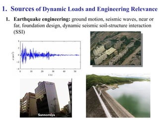
  • 1. 1. Earthquake engineering: ground motion, seismic waves, near or far, foundation design, dynamic seismic soil-structure interaction (SSI) 1. Sources of Dynamic Loads and Engineering Relevance 5
  • 2. 6 3. Blast and shock engineering: refinery design, homeland security, defense industry, air and ground shocks, explosion, mining, ... 2. Wind engineering: high-rises, long bridges, transmission towers, tall chimneys
  • 3. 7 4. Dynamic foundation design or foundation isolation of machines/equipment: pump stations, compressors and turbines, high- tech buildings, wind turbines, … 5. Pile driving & capacity: impact and stress waves, hammer cushions, bearing capacity determination, NDT, ‘wave equation’ method
  • 4. 6. Impact loading transmitted to foundation and structures 8
  • 5. 9 7. Offshore foundation engineering 8. Geophysical methods & in-situ sounding
  • 6. 9. Dynamic design for high-speed transportations, tunnels, buried pipelines 10 10. Construction induced vibrations ….
  • 7. 2. Theory of Dynamics & Vibrations Basic principles: • Newton’s laws in physics • Free-body diagram for dynamic problems 2 types of systems: • Discrete systems (finite number of degree of freedoms) • Continuous systems (infinite d.o.f.s) 11 . ., 2 : nd e g law m   F a m   i f a
  • 8. Discrete systems (finite number of degree of freedoms) • Lumped mass system: (a) Single or 1-dof system 12 x(t) f(t)
  • 9. (b) Multi-dof system (c) Continuum system 13
  • 10. 14 Analysis of a Single d.o.f. system (SDOF): (a) sign convention (b) Free-body diagram (FBD) for x(t) f(t) m k c (c) Write the equation implied by FBD: ( ): ( ) LHS RHS f t k x c x m x           ( ) m x c x k x f t      … a simple 2nd-order differential equation cx  kx = m x  f(t) m i F a  
  • 11. 15 1st step: Free Vibration Problem: Common canonical form of the ‘Equation of Motion’ by dividing by m, .... a 2nd-order homogeneous differential equation 0 m x c x k x      2 2 0 ................ (*) n n x x x        .......... ( / ) .......... 2 2 2 2 ...... n n c n k where circular rad s m c m k c m m km m natural frequency fraction ofcritical damping / damping ratio Critical damping constant                 
  • 12. Solution of Take • Special case 1: =0 (i.e., undamped case) 16 2 2 0 ......... (*) n n x x x        2 2 (*) ( 2 ) 0 t n n A e         2 2 2 1,2 For non-trivial solution, must have ( 2 ) 0 .............. a simple quadratic equation whose 2 roots are 1 n n n n                1,2 1 , , = 1 n n i i          ( )= ' ' n n i t i t x t a e b e      cos( t) sin( t s ) cos in n i t n i n e i e i             Recall     ( )= ' cos( t)+ sin ( t) ' cos( t)- sin ( t) ( ' ')cos( t) ( ' ')sin ( t) = cos( t) sin ( t) ! n n n n n n n n x t a i b i a b i a b a b               ( ) t x t A e 
  • 13. 17 ( ) cos( ) sin( ) (*) sin( ) sin cos cos sin . n n x t a t b t trigonometricidentity A A A              General solution : ( ) ( ) 2 2 / ... "natural period" 1/ ... "natural frequency" ( / sec) 2 ... " natural frequency" ( / sec) / ....( / sec) n n n n n n n n n n t T t T f T Hz cycle f circular rad with k m rad                    2 2 (*)... , sin cos , (*) ( ) where " " , " " . To determine the 2 constants ( , ) or ( , ) in the general solution, n n Taking t a A and b A then is equivalent to x t A t a A a b b a b A                   -1 = sin( + ) amplitude = phase angle = tan use initia 0 0 : (i) initialdisplacement x(0)= x (II) initialvelocity x(0) = x l conditions  
  • 14. Case (ii) >1 (over-damped case) 18 both are pure exponential decaying terms (no oscillation at all) 2 1,2 1,2 are both -ve from 1 n n          1 2 ( )= t t x t a e be       Case (iii) =1 (Critically-damped case) 1 2 = ( . . ) n i e a double root          1 ( )= +b +b n t t x t a t e a t e      
  • 15. 19     2 2 2 2 1 1 1 1 ( )= ' ' ' n n n n n n n n i t i t i t i t t t x t a e e a e e b e e                             Case (iv) 0 <  < 1 (Under-damped case) - most relevant to geotechnical & structural problems 2 2 1,2 1 1 n n n n                i 0 0 As in previous cases, can find the 2 constants : 1) initialdisplacement x(0)= x 2) initialvelocity x(0) = x by initial conditions         2 2 1 1 2 = ' ' = ' ' sin ( ) 1 ... " " n n n n d d n i t i t t t i t i t t d d n e a e b e e a e b e e A t where damped natural frequency                              
  • 16. 20 0 0 Imposing theinitial conditions of (1) initialdisplacement x(0)= x , (2) initialvelocity x(0) = x , one finds  
  • 17. Applications: Determination of damping ratio by Logarithmic Decrement method (for small ) 21 1 1 from solution, n N n N t N t N x Ae x Ae Note : free vibration zw zw        1 1 ( ) 1 n N n N N n N t t t N t N x e Then e x e zw zw zw               nt Ae zw 
  • 18. 22 ᇱ ே ேାଵ ௡ ேାଵ ே ௡ ௗ ௗ ௗ ௗ ௡ ଶ ଶ
  • 19. (II) Forced vibration 23 ( ) m x c x k x F t      2 2 ( ) / ................ (*) n n or x x x F t m        0 0 Consider a common and basic form of dynamic load: ................ (*) .... force magnitude .... excitation frequency ( ) sin( ) F F t F t     homog particular ( ) ( ) ( ) x t x t x t   General Solution to (*): ( ) ( ) forced vibration free vibration or x t x t  
  • 20. 24 : sin( ) cos( ) Take A t B t P f P To find x (t) or x (t) x (t)         2 2 2 2 0 2 2 0 2 2 2 sin( ) ( 2 )cos( ) ( / )sin( ) / 2 0 2 n n n n n n n n gives A B A t B A B t F m t A F m B                                                      2 P n P n P 0 Equation of motion x + 2ςω x +ω x = F / m sin(ωt)   2 2 cos( ) sin( ) sin( ) cos( ) then A t B t then A t B t P P x (t) x (t)                            2 2 0 2 2 2 2 2 2 2 2 2 2 0 . / 2 det / 2 0 / det / 2 2 0 n n n n n n n n F m A F m B                                         2x2 equations :Solution is (e g. by Cramer's rule) [ ] [ ]
  • 21. 25                             2 2 0 2 2 2 2 2 2 2 2 2 2 0 2 2 2 2 2 2 0 2 2 2 2 0 2 . / 2 det / 2 0 / ( ) / 2 / det / 2 2 0 2 / / 2 n n n n n n n n n n n n n n F m A F m F m B F m x2 equations : Solution is (e g. by Cramer's rule)                                                                         2 0 2 2 2 0 2 2 2 / (1 ) 1 2 / 2 1 2 n F k A F k B with                           where                                          0 n P 2 2 2 2 n n n ω 2ς F / k ω x (t) = sin(ωt - ) tan = ω ω ω 1 - 1 - + 2ς ω ω ω sin( ) cos( ) in A t B t     P x (t)
  • 22. 26     1 ( , ) w h ere S x                                                               0 P 2 2 2 n n 0 2 2 2 n n n n F / k x (t) = sin (ω t - ) ω ω 1 - + 2 ς ω ω D y n a m ic A m p lifica tio n F a cto r Q u a si - S ta tic D eflectio n ω A .F . ς F / k ω ω ω 1 - + 2 ς ω ω ω 2 ς ω ta n f = D e in itio n s :        2 n ω 1 - ω : this means the forced response amplitude is • ( , ) P S n Note x x AF    
  • 23. 27
  • 24. Half-power method for  using steady-state vibration test data 28 / 1 max max and ark a horizontal line with and find its 2 intesection points 2 with the AF curve and their corresponding frequencies and 1. Identify peak/natural frequency peak amplitude 2. M peak natural A A w w Steps : 2 2 1 . - 3. Then 2 2 peak peak w w w w V w w D  ;
  • 25. 36 A simple example of application: Base isolation design for foundation 0 ( ) sin( ) ground motion y t y t   ( ) absolute displacement w.r.t. a fixed frame x t  Free-body diagram: = ( ) k x y  ( ) c x y    m x 
  • 26. 37 FBDgives the equation: ( ) ( ) k x y c x y mx         0 0 ) Keeping unknown terms on LHS and prescribed term on RHS, one gets ( ) sin( ) cos( ) .................(* mx cx kx k y c y t y k t c y t                 2 2 0 0 sin( ) ( ) ky c y t F t        0 Recall the forced response amplitude is • ( , ), / P S S x x AF x F k                 2 2 2 2 0 0 0 0 2 2 0 max 2 2 2 For (**), . 1 / Thus 1- 2 p n n F ky c y y k c y c k x                                          2 2 2 2 0 1 2 1- 2 2 n p Max n n crit x y noting c k m                                                    Ground motion transmissibility
  • 27. Ground motion transmissibility & design implications: 38
  • 28. Dynamic Analysis by Complex Notation 39 Recall cos( ) sin( ) i t e t i t        0 0 2 0 = (cos( ) sin( )) or 2 .... (*) / i t i t n n t i t x x x m x c x k x F e F F m e              Consider     Take ( )=X ei t x t   Solution : 2 ( )=i X e , ( )= X e ! i t i t x t x t                 0 2 2 0 0 2 2 2 (*) ( ) ( 2 ) 2 ( 2 ) 1 / n n n n n n t i hen gives m whose solutio i X n is X i k F F m F                                                        Note: 1 its form is a ib 
  • 29. 40 0 2 2 2 2 2 2 2 2 : 1/ 1 2 1 2 1 1 2 1 2 n n n n n n n n Note k X i i k F                                                                                                                                                                 0 F   
  • 30. 41 0 0 2 2 0 0 1 ( ) ( ) ( )* (1 ) 2 ( ) is called the function. Inversely, (1 ) 2 ( ) ( n n n n k X X F i where k i X or F or F F                                                                                               C C Dynamic Compliance K ) ( ) is called the / function for the model. X where  Dynamic Impedance Stiffness K i t F e   ( ) i t x t X e    ( )  C
  • 31. 42 0 0 0 0 : ( ) ( ) F sin(ωt) which is the of . then the corresponding response x(t) must be the Imaginary part of X . ( ) ( ) F cos(ωt), which is the of . then th i t i t i t a If F t F e e b If F t F e      Results imaginary part real part e corresponding response x(t) must be the Real part of X i t e  0 = (cos(ωt)+isin(ωt))as to the equation of moti a forced excitation of (cos(ωt)+i sin(ωt)), with i.e., now we got the solution F i t X X e 0 2 2 0 2 2 2 2 2 2 / 1 2 1 2 1 2 1 2 ( ) i t i t n n n n n n n n k X e e i i k F x t F                                                                                                                                                            (cos(ωt)+i sin(ωt))           
  • 32. 43 2 0 2 2 2 2 2 2 , 1 2 ( ) ( * ) sin( ) cos( ) 1 2 1 2 i.e n n i t n n n n x t X e t t k F                                                                                                                                    0 For F(t) = sin(ωt) Im F ., exactly the same result we had before!
  • 33. Method of Fundamental Solution (Duhamel integral) for arbitrary forcing for SDOF 44  f() t  f(t) Concept: consider the loading as a sequence of many small impulses. Tool needed: a Unit-impulse response function g(t,) which gives the displacement of a dynamic system due to an impulse of unit magnitude at time  with zero initial conditions. 1 0 We can then write ( ) ( , ) ( ) In the limit of & 0, ( ) ( , ) ( ) N i t x t g t f N x t g t f d                    f() t
  • 34. 45 Next, need g(t,): : ( ) ( ) . 0 for t except 0 , ( ) 0 ( ) 1 . Solution m x c x k x t or m g c g k g t with zero initial conditions at t In the above the function t at t t dt is called the                                          deltafunction     t 1/ 
  • 35. 46 (1) 0 , For t    0 m g c g k g      with zero initial conditions (2) , 0... ! For t m g c g k g free vibration problem also        ( , ) 0 g t    . o let's use the general free-vibration solution of ( , ) sin( ) . nt d But likely non zero conditions at t after the impulse at time S g t A e t for t              
  • 36. 47   + + (3) Theimpulse effect going from t= to : : Consider ( ) Idea m g c g k g t dt                + + + + + : 1st term: ( , ) 2nd term ( , ) 0 3rd term ( ) 0 LHS m g dt m g m g m g dt m g m g m g dt m g dt m g                                               + : ( ) 1 RHS t dt        
  • 37. 48 LHS: 1 ( , ) 1 ( , ) ( , ) 0 m g or g m g                ( ) : 0 ( , ) 1 sin( ( ) n t d d Summary for t g t e t for t m                         ( ) 0 giving the solution under arbitrary forcing as 1 ( ) sin( ( ) ( ) . n t t d d x t e t f d m the              Duhamel Integral 1 0 d A m    
  • 38. Practical Numerical Evaluation of 49 ( ) 0 1 ( ) sin( ( ) ( ) for arbitrary ( ) n t t d d x t e t f d f t m              ( ) 0 0 ( ) sin( ( ) sin( )cos( ) cos( )sin( ) ( ) sin( ) cos( ) ( ) cos( ) ( ) sin( ) ( ) n n n n n n n d d d d d t t t t t t d d d d d d Note i t t t ii e e e e t e t x t e f d e f d m m                                                  The two integrals can be numerically by trapezoidal rule or Simpson rule for arbitrary ( ). f t Remarks: 1. Good for arbitrary loading 2. Dumhamel integral (a convolution integral) 3. A time-domain method (vs frequency-domain methods)
  • 39. Numerical Step-by-Step Time Integration Methods  Direct time-domain procedures  Allow for nonlinear problems (e.g., a change in k, c, or m as a function of time and deformation)  Arbitrary loading time function  Variety of algorithms and propoals  Commonly used in FEM, FDM, BEM  Underlying numerical and discretization issues 50 x(t) f(t) m k c f(t) t t
  • 40. 51 Idea: f(t) t t x(t) t t t x x x             t+ t x x x              forcing t+2 t x x x              forcing ( ) . m x c x k x f t with some prescribed initial conditions      t t+t
  • 41. 52 Assumption: the acceleration varies linearly in the time interval of t.  Example : Linear acceleration method : Writing ( ) , ( ) , ( ) , the assumption ( ) 0 t t t t t t t x t x x t x x t x x x x t x for t t                               0 2 ( ) ( ) 2 t t t t t t x t x x t d x x x x t                                  0 2 3 ( ) ( ) 2 6 0 . t t t t t t t x t x x t d x x x x x t for t                                      t x  t t x   t t   t
  • 42. 53 Taking = t, eq (1),(2), (3) become   ( ) (1) t t x x t t       ( ) (2) 2 2 2 t t t t t t t t t t t t t t x x x t x x x x x                       2 2 (3) 3 6 t t t t t t t t x x x t x x              i.e., the primary unknown is t t x   To find it, ( ) ( ) ! t t t t t t t t m x c x k x f t at t t m x c x k x f t                 
  • 43. 54 ( ) t t t t t t t t m x f t c x k x          2 2 ( ) ( ) ( ) 2 2 3 6 t t t t t t t t t t t t t t t f t c x x x k x x t x x                       2 2 , [ ] ( ) ( ) ( ) 2 6 2 3 t t t t t t t t t Collecting the terms t t t t m c k x f t c x x k x x t x                     2 2 1 leading to [ ] ( ) ( ) ( ) (*) 2 6 2 3 t t t t t t t t t t t t t x m c k f t c x x k x x t x                            
  • 44. 55        1 1 With and computable bymeans of (2) and (3) upon obtaining , one can collectivelydetermine the displacement, velocityand acceleration at according to w [ ] [ ] t t t t t t t t t t t x x x t t           x f B x A A       here upon defining . [ ], t t t t x x x and            x B f A   2 This is a step-by-step algorithm by which .... ! t t t t t t n t x x x x x x x x x x x x                                                        
  • 45. 56 Note: 1) Concept of stability, accuracy, efficiency a) Conditionally and unconditionally algorithms: a critical time step tcrit if conditionally stable. b) Accuracy: Level of numerical amplitude decay/damping & phase shifts due to accumulation of errors. c) Explicit and Implicit schemes. d) Short duration versus long-duration problems. e) Applicable to MDOF systems (see posted reading) a) Other methods e.g., Central difference, Newmark method in many commercial FEM codes (see posted reading)
  • 46. 5 Response Spectrum (a spectral method) The maximum response of a Single degree of freedom system with general to a specific excitation (e.g., earthquake ground motion) : ( , ) n     2 2 ( ) g n n g c x k x m x x or x x x x t                 = -kx-cx m (x+ x ) g    ( ) g x t  / g x g 
  • 47. 6 ( ) 0 ( ) 2 0 Analytically, thedisplacement response is expressible in the Duhamel integralform as 1 ( ) sin( ( ) ( ) 1 sin( ( ) ( ) ..... (*) 1 n n t t d d t t d g n x t e t f d m e t x d                               max v pv ( ) ( , ) .... ( , ) .... d d x t S S      Spectral velocity Spectralpsuedo velocity     ( ) 0 1 ( ) ( ) sin( ( ) ( ) n t t d g d d b x t e t x d dt                   ( ) pv max 0 ( , ) sin( ( ) ( ) is n t t n d g S e t x d called               SpectralPsuedo- Velocity  Leibniz rule :   0 0 0 ( , ) ( , ) ( ) ( , ) ( ) ( ) ( , ) ( ) t t g g g t g d dt g t g t x d g t t x t x d dt dt t g t x d t                           a max (c) ( ) ( ) ( , ) ... g d x t x t S     Spectralacceleration   max pv ( ) ( ) ( , ) .... 1 ( , ) d d n n a x t S S where       Maximum response quantities : Spectral Displacement 
  • 48. 7     : eqn of motion g gives m x x c x k x     Note       max max 1 g implies x x c x k x m          2 max g n d n k x x S m        d pv S S   Summary of Approximate relations of Spectral displacement, velocity and acceleration to Spectral pseudo-velocity d pv n V pv a n pv 1 S = S ω S = S S = ω S 2 n n with T   
  • 49. 8 2 2 n n T T     d pv pv n V pv a n pv pv 1 S = S S ω S = S S = ω S S log log log log(2 ) log log log log(2 ) n n T T           d pv a pv S S S S y = m x +b Line of constant Sd Line of constant Sa
  • 50. 9 Tripartile plot of response spectrum
  • 52. 11 Frequency domain analysis 0 0 0 1 0 0 Recall for periodic functions of period T: 2 2 f(t)= sin( ) cos( ), ( ) n n n n a n t b n t or T T                Fourier series 0 0 0 0 0 0 0 0 where f(t) sin( ) f(t) cos( ) n n a n t dt b n t dt                     0 0 0 0 / 0 / A much more compact form is f(t)= = f(t) 2 in t in t n n n F e with F e dt                 0 0 0 0 / 0 / or f(t)= = f(t) 2 in t in t n n n F e with F e dt                 t f(t)
  • 53. 12 0  0 2 0  0 3 2 2 n n a b  Can determine the phase angle of magnitude of each sinusoidal component of f(t) ie f(t) can be looked upon as a sum of sin( ) ! n n n A n t    Can determine the amplitude/magnitude of each sinusoidal component of f(t) as 2 2 n n a b 
  • 54. 13 ( )= f(t) i t F e dt        (e.g. an earthquake ground motion or response) Next : How to treating as non -perioidc function? 0 0 0 0 2 ( ) , ( ) / , ( ) , ( ) ( ) n a d b c n d F F T                  1 f(t)= ( ) 2 i t F e d         0 1 1 then (*) becomes f(t) ( ) (2) 2 2 in t i t n n F e d F e d                  The Fourier transform of f(t) Inverse Fourier transform of ( ) F   0 0 0 0 / 0 / Note that 1 f(t)= = f(t) (*) 2 in t in t n n n F e with F e dt                 In the limit of T   leading to
  • 56. 15 Remarks:  is generally a complex-valued function of frequency, i.e., with a real and an imaginary part.  is the Fourier amplitude spectrum (real value)  Exposes the frequency content of the loading or response  It is a full characterization of f(t) in the frequency domin  i.e.,  FFT algorithms (Fast Fourier Tranform) ( ) gives ( ) and ( ) gives back ( ) ! f t F F f t completely     ( ) F   ( ) F  
  • 57. 13 ( )= f(t) i t F e dt        (e.g. an earthquake ground motion or response) Next : How to treating as non -perioidc function? 0 0 0 0 2 ( ) , ( ) / , ( ) , ( ) ( ) n a d b c n d F F T                  1 f(t)= ( ) 2 i t F e d         0 1 1 then (*) becomes f(t) ( ) (2) 2 2 in t i t n n F e d F e d                  The Fourier transform of f(t) Inverse Fourier transform of ( ) F   0 0 0 0 / 0 / Note that 1 f(t)= = f(t) (*) 2 in t in t n n n F e with F e dt                 In the limit of T   leading to A Fourier transform pair
  • 59. 15 Remarks:  is generally a complex-valued function of frequency, i.e., with both real and imaginary parts.  is the Fourier amplitude spectrum (real value)  Exposes the frequency content of the loading or response  It is a full characterization of f(t) in the frequency domin  i.e.,  FFT algorithms (Fast Fourier Tranform) ( ) gives ( ) and ( ) gives back ( ) ! f t F F f t completely     ( ) F   ( ) F  
  • 60. 16 Basic operational properties: Fourier transformof derivatives: [ ( )] ( ) ( )= ( ) w w ¥ - -¥ Á = = ò   i t recall f t f t F f t e dt ( ) ( ) 2 ( ) [ ( )]= ( ). [ ( )] ( ) w w w w ¥ - -¥ Á = Á = ò     i t d b f t f t e dt dt i f t i F F ( ) ( ) ( ) [ ( )]= ( )! w w Á  n n c f t i F ( ) In integration by part, ( ) ( ) ( ) ( ) ( ) ( ) 0@ w w w w w w w - ¥ - -¥ ¥ ¥ - - -¥ -¥ = - = + =  ¥ ò ò  i t i t i t i t de f t e f t dt dt f t e i f t e dt i F if f t ( ) ) [ ( )]= ( ) ( )= ( ) w w w ¥ ¥ - - -¥ -¥ Á = = ò ò      i t i t df t a Consider f t f t F f t e dt e dt dt
  • 61. 17 : ( ) Solution of SDOF equation of motion under arbitrary forcing m x c x k x f t    Applications :     To apply Fourier tranform method, consider ( ) i t m x c x k x f t e dt       2 ( ) ( ) ( ) m i c k X F                2 ( ) ( ) ( ) ( ) ( ) ( ) ( ) ( ) ( ) . i t with i m X i c X k X F X x t e dt as the Fourier tranform of x t etc                        ( ) i t m x c x k x f t e dt         
  • 62. 18 2 ( ) ( ) 1 X F m i c k                  or 2 2 ( ) / ................ (*) n n x x x f t m          2 2 ( ) ( ) (*) ( ) 2 / n n then gives i X F m               2 2 2 ( ) ( ) ( ) ( ) 2 1 (1 ) 2 n n n n m X i k i F F                                                                      
  • 63. 19 2 : : . : 2 ( ) n n g Example Earthquake ground motion problem Eq of motion x x x x t              2 2 / ( ) ( ) ( ) ( ) 1 ( ) 2 n n x x X x i x                       H       Concept of a Transfer function Excitation Response Transfer function H()
  • 64. 19 2 : Earthquake ground motion problem: . : 2 ( ) n n g Recall Eq of motion x x x x t Example -             2 2 / ( ) ( ) ( ) ( ) 1 ( ) 2 g n n x x g X x i x H                             Concept of a Transfer function Excitation Response Transfer function H() of dynamical system
  • 65. 20  ( ) g x w    ( ) X w   ( ) w H
  • 66. 21 Remarks:  Theoretical modeling characterization of dynamic and vibratory systems in frequency domain  Other transfer functions of engineering interest / v/ / ( ), ( ), ( ) . ., g g g d a a a a e g H H H     Experimental determination of transfer functions of physical systems
  • 67. 22  ( ) w H In more complex systems:
  • 68. 23 2 : (2 ) g n n a x x x x Note           2 (2 ) n n a x x           : : ! g g g a x x a x x Note a x x Note                      2 2 ( ) ) 1 ( ( ) ( ) 2 n n With X i x                        2 2 2 ( ) 1 ( ) 2 n n a x i                             2 2 2 ( ) 2 ( ) 2 n n n n i a x i                          Re Im Z1+ Z2 Z2 Z1
  • 69. Half-power method for  using steady-state vibration test data 28 / 1 max max and ark a horizontal line with and find its 2 intesection points 2 with the AF curve and their corresponding frequencies and 1. Identify peak/natural frequency peak amplitude 2. M peak natural A A w w Steps : 2 2 1 . - 3. Then 2 2 peak peak w w w w V w w D  ;
  • 70. Method of Energy Balance 29   2 2 1 1 ( ) 2 2 Kinetic energy m x Potential elastic Energy k x For a 1DOF :   & x(t) f(t) A B 0 ( ) sin( ) ( ) sin ( F t F t x t A t for + ) undamped free vibration           2 2 2 2 Note that KE+PE= At time A, KE+PE=0 , 1 2 1 At time B, KE+PE= 2 0 2 1 1 2 n n n k A m A k k A m A m Conservation of energy w w w       constant for undamped case
  • 71. Method of Energy Balance 30 2 / 2 / 2 / 0 Idea: Compare Input nergy & energy dissipated per cycle ( ) sin( ), ( ) sin( ), ( ) cos( ) ( ) ( ) sin( ) T T T input o o o E F t F t x t A t x t A t dx W F t dx F t dt F t A dt p w p w p w w w f w w f w w D                 Damped 1DOF under Forced Steady State Vibration : &   2 / 0 2 / 2 0 0 cos( ) sin( ) cos( )cos( ) sin( )sin( )) sin( ) sin ( ) sin( ) T o T o t dt F A t t t dt F A t dt F A p w p w w f w w w f w f f w p f           x(t ) f(t)   2 / 2 / 2 2 / 2 ( ) ( ) cos( )) ..... T T dissip damping o o T o dx dx W F t dx t c dt dt dt c A t dt cA p w p w p w w w f wp D                   
  • 72. 31 0 2 0 os( ) sin( ) ................ (*) : input dissip input dissip W W W F Ac For steady state must ha W c A F A c ve p f pw f w D D D D      0 2 max 2 2 / C a (*) is ident : ical t - o l 2 im 1 p n n F k x w w V w w                             
  • 73.   Hysteretic cyclic stress-strain behavior in many real materials 32 Area  energy dissipation
  • 74.   Linear viscous model vs physical cyclic stress- strain behavior : 33 Hysteretic loop’s area’s strong frequency dependency in linear viscous damper not seen in real materials x F
  • 75. Equivalent Viscous Damping 34 exp 2 exp 2 ( ' ) ................ (*) erim dissip erim W c A W hyster loop s area W and define ak A T e equiv Idea c : pw pw D D D    2 2 exp 2 2 (2 ) (2 ) 2 equiv equiv erim crit crit crit equiv n n equiv n c c W c Ta A c A km c A km A ke k Minor - arrangement : pw pw w z p w w w p z w D           exp 2 ! 1 4 2 erim equiv n W kA z w p w D               2 exp 1 4 2 erim equiv n W kA w pz w D             
  • 76. • If experimental measurement is done at 35 exp exp 2 ! 1 4 4 2 erim erim equiv W W Triangular Area kA z p p D D         n      A
  • 78. Shear Modulus and Damping: Stress‐strain response is hysteretic and strain level dependent Basic engineering parameters: ‐secant modulus G ‐equivalent viscous damping  both of which are dependent on level of confinement/stress state 2 1 4 2 loop equiv G Area G             
  • 79. • Soil is a particulate/porous medium • Under a water table, void space in the ‘soil skeleton, is filled by water with pore water pressure u SOLID GRAINS WATER
  • 80. Importance of effective stresses: They control: (a) Shear strength/failure condition in soil (b) Stiffness/deformability/settlement of foundations v v vertical soil effective stress horizontal soil effective stress h h u u           v h    Concept of Effective Stress in Soil u
  • 81. In 3D: Note: Sign convention in soil mechanics: Compressive stress is positive
  • 82.
  • 83. Field Measurement Methods: (I) For low  level (<10‐6 to 10‐4 ) ….. Gmax (II) Geophysical/wave‐based methods (downhole, cross hole seismic measurements) (III) Impulse or low‐level vibration methods (IV) Shear wave speed: Compressional P‐wave speed: 2 1 1 2 p G V             s G V  
  • 84. Typical range of Vs: 200’/s to 1500’/s for unconsolidated soil. 2000’/s for stiff soils 3000’/s for sandstone >6000’/s for rocks E.g., =100 lb/s, Vs=300/s: Gmax =(100/32.2)(300)^2 = 0.28x10⁶ lb/sqft(psf) Gmax =(100/32.2)(1500)^2 = 7x10⁶ lb/sqft(psf) 1psf=47.85Pa 1 psi=6.891 kPa
  • 85. DIFFERENT LABORATORY TESTS FOR DIFFERENT STRAIN LEVELS
  • 86.
  • 87. Laboratory methods: Resonant column tests: ‐excited torsionally (or axially) at the top or base into resonant modes ‐transducers used to measure motion’s time histories ‐sinusoidal or random excitation ‐use of solid or hollow samples ‐ Equiv viscous damping ratio from hysteretic loop (r)
  • 88.
  • 89. Lab tests for higher strain level: (a) Cyclic simple shear test Can be stress‐control or strain‐controlled Drained or undrained (pore pressure development) Simple shear (stack rings) vs direct shear test cyclic h0  cyclic  v0 (v0 ,‐cyclic) (h0 ,cyclic)
  • 90. (b) Cyclic triaxial test: Repetitive axial compression/extension ‐ different stress path stress control or strain controlled Drained or undrained (pore pressure development) 0  0+d‐cyclic  d‐cyclic (0 ,0) , , 2(1 ) E E G G          ~ 0.15 to 0.35 (sand) 0.5 (saturated clay)  
  • 91. (c) Bender element test Piezoelectric sensors (transmitter and receiver) Measure average wave speed between 2 points in specimens s measured L G V t      + ‐
  • 92. (d) Shake Table Test others….
  • 93. Experimental Synthesis and empirical relationships:  Gives trends with respect to basic factors  Different functional forms proposed  Useful for preliminary assessments
  • 94. Primary factors affecting shear modulus & damping ratio Strain amplitude Mean effective stress Void ratio Relative density Dr (sand) Secondary factors # of cycles, OCR,  & c, grain characteristics, soil fabric & structure, frequency, degree of saturation, cementation
  • 95. Empirical relationships on shear modulus:  Useful for preliminary assessments  Gives trends with respect to basic factors     1/2 2 max 1/2 2 . ., (1972) (2.973 ) 1230 ... angular grains 1 1 ( ) ( ~ ) (2.17 ) 2630 ... round grains 1 1 0 0 20 .18 40 .30 60 .41 k mean k mean e g e OCR e psi G psi e OCR e psi PI k where -4 Hardin & Drnevich 10                                                    
  • 96. units of G and p = kg/cm2 Iwasaki et al. (1978)
  • 97. 1/ 2 2 4 2 0..44 2 2 5 max 2 0..4 2 6 2 (1978) (2.17 ) 700 , @10 1 1 / (2.17 ) ( / ) 850 , @10 1 1 / (2.17 ) 900 , @10 1 1 / mean mean mean e e kg cm e G kg cm for sand e kg cm e e kg cm                                                            Iwasaki et al
  • 98. Seed and Idriss (1970) Separate sand and clay         1/ 2 max 2 2 max max 2 max ( ) 1000 , 15 0.6 , 1 0.6 , 2 ,.... ( / ) ( , ) mean u G psf K K Dr F psf F for silt F for gravel G kg cm f OCR PI S Sand : Clay :               𝐾
  • 99.
  • 100. Strain dependence of cyclic shear modulus • Basic observations: (a) γ τ γ m m c g g t = + max ( ) , i As g t t  ¥  m c g t g  = + max 1 m t  =
  • 101. max 0 ( ) 0, d i As G d g t g g =   ( ) 2 1 d m d m c m c t g g g g æ ö æ ö ÷ ç ÷ ç ÷ ç ÷  = - ÷ ç ç ÷ ÷ ç ÷ ç ç + ÷ è ø ç + è ø max 0 1 d G d c g t g =  = = 1 1 1 ( ) ( ) max max max max max G G G G G g g g t g t = +  = + Summary : ( ) 1 1 1 1 max ref max max max ref max G where G G G t g g g g g t  = = = + +
  • 104. Basic observation: (b) 1 (i) reverse slope Gmax (ii) half area of loop constant% * triangle a_b_c’s area triangle abc’s area k » » =  max 1 triangle abc’s area= (ad)(cd-cb) 2 where ad =2 2 / 2 / cd G bd G t t t ⋅ = = 2 1 1 max max 1 1 1 1 area of hyeteretic loop= (2 )2 = 4 k k G G G G t t t æ ö æ ö ÷ ÷ ç ç ÷ ÷ ⋅ - - ç ç ÷ ÷ ç ç ÷ ÷ ç ç è ø è ø 2 1 1 max 2 max max max 1 1 4 2 ( ) = 1 1 4 ( 2 ( ) 1 k k G G G Equivalent damping ratio G G G G t g t p p g z z æ ö ÷ ç ÷ - ç ÷ ç æ ö ÷ ç è ø ÷ ç ÷ = - ç ÷ ç ÷ ç è ø æ ö ÷ ç ÷  = - ç ÷ ç ÷ ç è ø
  • 106. Concept of Strain‐compatible shear modulus and damping To recognize the significant strain‐dependence of the shear modulus and damping ratio, one generally needs to use a pair of G and  in the dynamic analysis of the model so that their values are consistent with the strain/deformation level of the response. Approach: 1. Assume an initial estimate of strain, say, 0 & obtain G(0) and  (0). 2. Perform dynamic analysis to find the predicted strain level, say, 1. 3. Check if 1 ‐ 0 is close enough. 4. If not, replace 0 by 1 and repeat step 1 to 4 until difference of the different n+1 and n is acceptable 5. Then G( n+1) and  (n+1) are called the Strain‐compatible shear modulus and damping ratio. * The iterative approach is built in the program SHAKE 91, 2000 for 1‐D equivalent linear ground response analysis 1 ( ) 0 max G G g 1 0 ( ) max z g z 0
  • 107. Multi‐Degree of Freedom Systems  Soil layering and profile variation  Improve accuracy and lower degree of approximation  Higher‐order wave motion at high frequencies
  • 108. Multi-D-O-F system  Continuum system 2
  • 109. m1 f1(t) x2(t) f2(t) H/2 H/2 , G , 2G FBD for Equations of motion for undamped case: x1(t) k1 k2 1 1 m x  f1 = 1 1 1 1 2 1 ( ) m x k x f x  + - =  1 1 2 ( ) k x x - 2 2 1 1 2 2 2 2 2 2 1 1 1 2 2 2 ( ) ( ) m x k x x k x or m x k x k x f f k  + = + - - - + =   f2 2 2 k x 2 2 m x  =
  • 110. FBD for Equations of motion for undamped case: 1 1 1 1 2 1 (1) ( ) m x k f x x + - =  2 2 1 1 1 2 2 2 ( ) (2) m x k x k k x f - = + +  { } { } { } In matrix form  [M] x + f = [K] x  { } { } 1 1 2 2 For the 2-DOF model of the soil layer, 0 .... 0 .... 3 , .... m Mass matrix m k k Stiffness matrix k k x f forcing vector x f é ù ê ú = ê ú ë û é ù - ê ú = ê ú - ë û ì ü ì ü ï ï ï ï ï ï ï ï = = í ý í ý ï ï ï ï ï ï ï ï î þ î þ [M] [K] x f Note: M and K are symmetric
  • 111. { } { } { } { } For a damped system, the equation of motion is + [M] x [C] x +[K] x f =   { } { } { } Case 1: Free vibration of undamped MDOF: + [M] x [ 0 = K] x  { } { } { } { } ) (0) ) (0) subject to a b = = Initial Conditions : x x x x   Note: Same matrix equation of motion from finite element methods
  • 112. { } { } { } { } For a damped system, the equation of motion is + [M] x [C] x +[K] x f =   { } { } { } Case 1: Free vibration of undamped MDOF: + [M] x [ 0 = K] x  { } { } { } { } ) (0) ) (0) subject to a b = = Initial Conditions : x x x x   Note: Same matrix equation of motion from finite element methods
  • 113. { } { } { } { } For a damped system, the equation of motion is + [M] x [C] x +[K] x f =   { } { } { } Case 1: Free vibration of undamped MDOF: + [M] x [ 0 = K] x  { } { } { } { } ) (0) ) (0) subject to a b = = Initial Conditions : x x x x   Note: Same matrix equation of motion from finite element methods
  • 114. { } { } { } { } For a damped system, the equation of motion is + [M] x [C] x +[K] x f =   { } { } { } Case 1: Free vibration of undamped MDOF: + [M] x [ 0 = K] x  { } { } { } { } ) (0) ) (0) subject to a b = = Initial Conditions : x x x x   Note: Same matrix equation of motion from finite element methods { } { } As in SDOF: ! i t e w I = dea : x η
  • 115. { } { } { } [ ]{ } { } [ ] { } [ ] 2 2 where the matrix For non-trivial solution of , must have det 0. or one w w  - + = é ù = - + ê ú ë û = ) = [M] η [K] η 0 H(ω η 0 H(ω) [M] [K] η H(ω) [ ] [ ] 2 2 2 2 2 2 0 For the 2-dof example, 0 3 3 with the determinant det ( )( 3 ) m k k m k k m k k k m k m k m k k w w w w w é ù é ù é ù - - + - ê ú ê ú ê ú =- + = ê ú ê ú ê ú - - - + ë û ë û ë û = - + - + - H(ω) H(ω)
  • 116. [ ] ( ) ( ) 2 4 2 2 2 1 2 2 Settingdet 0 4 2 0, a quadratic equation in . : (2 2) 0.585 (2 2) 3.414 Theyare the of t k k m m k k Roots m m k k m m w w w w w æ ö æ ö ÷ ÷ ç ç =  - + = ÷ ÷ ç ç ÷ ÷ ç ç è ø è ø æ ö æ ö ÷ ÷ ç ç = - = ÷ ÷ ç ç ÷ ÷ ç ç è ø è ø æ ö æ ö ÷ ÷ ç ç = + = ÷ ÷ ç ç ÷ ÷ ç ç è ø è ø H(ω) naturalfrequencies 1 he MDOFsystem. Put in ascending order, the lowest frequency, i.e., is called the Fundamental natural frequency. w
  • 117. Modal shapes associated with each natural frequency { } { } { } ( ) ( ) { } ( ) 2 1 1 1 1 2 : ... (*) will allow non-unique solutions 2 , (*) 1 2 1 1 2 0 normalize it in 0 1 1 2 1 For a For the dof system can be reduced to or w w h h é ù - + ê ú ë û é ù ì ü - + - ï ï ì ü ì ü + ê úï ï ï ï ï ï ï ï ï ï ï ï ê ú =  = í ý í ý í ý ï ï ï ï ï ï ê ú ï ï - + î þ ï ï ï ï î þ ï ï ê ú î þ ë û 1 1 1 [M] [K] η = 0 η η { } { } { } ( ) ( ) { } ( ) 2 2 2 2 1 2 different ways : will allow non-unique solution 1 2 1 1 2 0 0 1 1 2 1 For a w w h h é ù - + ê ú ë û é ù ì ü - + - ï ï ì ü ì ü - ê úï ï ï ï ï ï ï ï ï ï ï ï ê ú  =  = í ý í ý í ý ï ï ï ï ï ï ê ú ï ï - + î þ ï ï ï ï î þ ï ï ê ú î þ ë û 1 2 1 [M] [K] = η 0 η η
  • 118. { } { } { } { } { } { } { } { } { } { } { } { } { } { } { } { } { } { } 2 2 2 2 ..... (1) ..... (2) 0 ..... (1) ..... (2) But since the matirx i i i j j j T T T j i j i j i T T T i j i j i j and is also true w w w w - + = - + = - + = = - + = Orthogonality of Mode Shapes Note : [M] η [K] η 0 [M] η [K] η 0 Observation : η [M] η η [K] η η 0 η [M] η η [K] η η 0 [K] { } { } { } { } { } { } ( ){ } { } { } { } { } { } 2 2 ! ( , too) is symmetic, it is always true that . , (1) (2) 0 0 , ! 0 T j i i j T j j i i j T i j i f and Ta i k f i g i n w w w w w w -  = = ¹ = -  ¹  T T T T [M] a [K] b = b [K] a a [M] b = b [M] η η [M] η η [K] a [M] η η { } { } We say that the mode shape with respect the the mass matrix and the stiffness matrix . i j is orthogon ] al η η [M t [K] o
  • 119. Usefulness: If we put the mode shape vectors in a matrix form { } { } { } { } { } { } { } 1 2 ... N T T i i ii T T i i ii then must be with the diagonal element must be with the diagonal element é ù = ê ú ë û  = L = = Q = [T] η η η [T] [K][T] [Λ] a diagonal matrix η [K] η [T] [M][T] [Θ] a diagonal matrix η [M] η . . diagonalizes both the ! i e and matrices [T] [K] [M]
  • 120. 0 & 0 3 1 2 1 1 2 1 2 , 1 1 1 2 1 m k k m k k é ù é ù - ê ú ê ú = = ê ú ê ú - ë û ë û é ù é ù + + - ê ú ê ú = = ê ú ê ú - ê ú ë û ë û T E.g. For the 2- DOF example of the 2- layered soil, [M] [K] [T] [T] ( ) ( ) 1 2 1 1 0 1 2 1 2 0 1 1 1 1 2 1 T m é ù é ù ê ú é ù é ù + + - ê ú ê ú ê ú ê ú = = = ê ú ê ú ê ú ê ú - ê ú ë û ê ú ë û ë û ê ú ë û 2 2 1+ 2 +1 0 [T] [M][T] m [Θ] 0 1- 2 +1 1 2 1 1 1 1 2 1 2 [ [ ] 1 3 1 1 1 2 1 T k é ù é ù é ù é ù + - + - ê ú ê ú ê ú ê ú = = = ê ú ê ú ê ú ê ú - - ê ú ë û ë û ë û ë û 4 0 T] [K][T] k Λ 0 4
  • 121. Modal Analysis of MDOF: Observation and Ideas: (i) If the mode shapes are orthogonal to each other. If so, they must be independent of each other! (ii) That means any x can be decomposed into a linear combination of the mode shapes , 1, 2 ..., i i N = η { } { } { } { } { } 1 2 1 2 1 2 1 . . ( ) ( ) ( ) ... ( ) ( ) .. N N N i i i N i e t q t q t q t q q q t q = = + + + ì ü ï ï ï ï ï ï ï ï ï ï ï ï é ù = = í ý ê ú ë ûï ï ï ï ï ï ï ï ï ï ï ï î þ å 1 2 N x η η η η η η ... η { } { } ( ) ( ) t t = i.e. let'swrite x [T] q The s are called the 'Principal' or 'Normal' coordinates of the dynamical system i q
  • 122. With , the equation of motion { } { } ( ) ( ) t t = x [T] q { } { } { } for free vibration of undamped MDOF becomes + [M] x [K] x = 0  ( ) t  + [M][T]q [K] = [T]q 0  ( ) ... (*) t + T T [T] [M][T]q [T] [K] = [T]q 0  ( ) ( ) ( ) ( ) ( ) ( ) ( ) ( ) 1 1 1 1 2 2 2 2 4 4 0 0 4 4 0 0 k m q k q q q m k m q k q q q m + =  + = - + =  + = - 2 2 2 2 1+ 2 +1 1+ 2 +1 1 2 +1 1 2 +1     1 1 1 1 0.5858 0 3.414 0 k q q m k q q m æ ö ÷ ç  + = ÷ ç ÷ ç è ø æ ö ÷ ç  + = ÷ ç ÷ ç è ø   ( ) 0! t + =  [Θ] q [Λ]q  [ ] T Now multiply it by T ( ) ( ) & [ [ ]! T T é ù ê ú é ù ê ú ê ú = = = = ê ú ê ú ë û ê ú ê ú ë û 2 2 1+ 2 +1 0 4 0 Recall [T] [M][T] m [Θ] T] [K][T] k Λ 0 4 0 1- 2 +1 2 1 1 1 1 2 2 2 2 2 0, . . ( ) 0, . . ( ) . ., ... (*) q q i e a SDOF for i q t q q i e a SDOF for q e gives t w w + = + =  
  • 123. 2 1 1 1 2 2 2 2 ( ) ( ) 0 ( ) ( ) 0 q t q t q t q t of w w + = + = Solution   i i A and B To find the constants , need Initial Conditions : { } { } { } { } { } { } ( ) ( ) (0) (0) (0) (0) t t =  = = Note x [T] q x [T] q x [T] q   { } { } { } { } 1 1 (0) (0) (0) (0) ! - - = = q [T] x q [T] x    1 1 1 1 1 2 2 2 2 2 ( ) cos( ) sin( ) ( ) cos( ) sin( ) q t A t B t q t A t B t w w w w = + = + 
  • 124. Forced Vibration of Undamped MDOF { } { } { } : (t) Equation of motion [M] x + [K] x f =  { } { } ( ) ( ) Take t t = Idea : x [T] q ( ) t n t he + [M][T]q [ [ = K T]q f ]  ( ) t T T T then [T] [M][T]q + [T] [K][T]q [T = f ]  ( ) t T then [Θ]q + [Λ]q [T] = f  1 1 ( ) t - - T then q + [Θ] [Λ]q [Θ] [T] = f  1 2 1 is diagonal with diagonal eleme t ( n s ! is called th ) e i where t w - -  = = T q + [Ω]q [P] [Ω] [Θ] [Λ] [P] [Θ] [T] Participation factor matrix = f  and each is called a ij P Participation factor
  • 125. Meaning of Pij : Pij gives an indication of how the forcing at the j th mass or node contribute to the vibration of the ith mode. 1 th 2 e.g., For the i mode's coefficient , ( ) ( ( ) ) N i i i i i j i j j q q t q P f t F t w = + = = å  1 1 2 2 3 3 ( ( ( . ( ) ) ) ) .. i i i iN N P f t P f t P f t P f t = + + + + { } { } { } { } { } { } { } 1 2 1 2 1 1 2 2 With ( ) ( ) ( ) ... ( ) one should note the entire product ( ) represents the 1st mode' contribution, ( ) represents the 2nd mode' contribution, etc to ( ) because the N N t q t q t q t that q t q t t = + + + ATTENTION : x η η η η η x { } size of depends the chosen normalization of . i i q η
  • 126. Damped MDOF system under Forced Vibration { } { } { } { } The equation of motion is + [M] x [C] x +[K] x f =   : Solution by modal analysis { } { } { } 1 2 2 1. Find ... from solving the eigenvalue poblem of [ ] 2. Take ( ) ( ) 3. Get [ ... (*) [ n t t w é ù = - + ê ú ë û = + +  + + T T T T T T [T] η η η M K η 0 x [T] q [T] [M][T]q T] [C][T]q [T] [K][T]q [T] f [Θ]q T] [C][T]q [Λ]q [T] f = = =   1 1 1 [ - - -  + + T T q [Θ] T] [C][T]q [Θ] [Λ] f = q [Θ] [T] 
  • 127. [ ] [ ] [ ] [ ] [ ] 1 1 0 ( ) ..... (*) ( ) ( ) ..... (**) N j j a b a b - - = = + = å Particulardamping forms that work : [C] M K Rayleigh Damping [C] M M K Caughey damping 1 1 1 4. 2 Will be diagonal generally? If Yes, can write it as 2 and treat the MDOF as N number of SDOF systems, i.e., [ i i etc z w z w - é ù ê ú ê ú ê ú ê ú ë û T T] [C][T] Key Question : [Θ] But the Answer is NO generally. 2 1 2 , 1,2,..., N i i i i i i ij j j q q q P f i N z w w = + + = = å  
  • 128. [ ] [ ] , a b = + For Rayleigh Damping [C] M K [ ] [ ] 1 1 [ [ [ [ [ then a a a a a - - - =  = = = = T T T Case 1: Mass proportionaldamping [C] M T] [C][T] T] M [T] Θ] [Θ] T] [C][T] [Θ] Θ] [I] [ ] [ ] 1 1 [ [ [ [ [ ....(**) then b b b b b - - - =  = = = = T T T Case 2 : Stiffness proportionaldamping[C] K T] [C][T] T] K [T] Λ] [Θ] T] [C][T] [Θ] Λ] [Ω] Equating to the diagonal matrix of 2 , 2 2 i i i i i i a z w a a z w z w  =  = [I] 2 Equating to the diagonal matrix of 2 , one gets 2 2 i i i i i i i b z w bw b w z w z =  = [Ω]
  • 129. [ ] [ ] 2 2 i i i a b bw a z w = + = + Rayleigh damping Case with [C] M K gives Modal damping ratio Note the difference in frequency dependency
  • 130. [ ] [ ] [ ] [ ] 1 1 2 ... ) is the ( N i i i ij j j N o wher r q q q P e f = ààà + + = = å -1 1 T T i i i i T T i i i i T - T [P] = [Θ] [T] [Θ] [ ] Partcipation Factor matrix η C η η K η η M η η M η η η η   [ ] [ ] [ ] [ ] [ ] ( ) ) 1,2,.., ( i i i q q q i N e à + àà + = = T T T i i i i i T T T i i i i i i η C η η K η η f η M η N η M η η M ot that can also be written as η   1 1 1 [ ( ) - - - + + à T T q [Θ] T] [C][T]q [Θ] [Λ]q [Θ] [T] = f   Modal form of governing equations for MDOF:
  • 131. 23 Importance of Modal Decomposition in dynamic analysis • One can choose/select only modes that are important to analyze (e.g., the lower modes in earthquake problems) • Can use larger time steps in using direct step-by-step integration methods (for stability and accuracy) • Without the modal reduction analytically, small time steps will be needed as all higher modes esp. for a complicated numerical model, are automatically included in the integration but high accuracy is not quaranteed . • Artificial numerical damping is thus often employed to damped out high frequency componentwsies
  • 132. 24 Particular Example: MDOF structures subject to Earthquake base motion
  • 133. { } { } { } { } Recall the general equation of motion for MDOF is: + [M] x [C] x +[K] x f =   { } { } ( ) a = Adaptation to earthquake ground motionproblem? f 0 { } { } { } { } 1 1 ( ) 1 1 ground b x where ì ü ï ï ï ï ï ï ï ï ï ï =í ý ï ï ï ï ï ï ï ï ï ï î þ abs x = x + 1 1    { } { } { } { } { } MDOF equation of motion for ground motion is ( ) ! ground x t effectively + = - [M] x [C] x +[K] x [M] 1 f =   
  • 134. { } { } { } { } With the Equation of motion for MDOF due to base ground motion ground x - + [M] x [C] x +[K] x [ = M] 1    [ ]{ } [ ] 2 2 ( ) i i i i i i grou i i nd o q q q x t w ere r h V w w a a æ ö ÷ ç ÷ - ç ÷ ç ÷ ÷ = ç è + ø T i T i i η M 1 + = η M η    { } 2 1 ! then by the modal decomposition via , one gets 2 ( ) i i i ground x t V w w - + + = =- T x = Tq q [ ]q [ ]q [Θ] [T] f [P]f [P] ] = [M 1    [ ] can be diagonalized by the modal shape/modal matrix , and assuming [C] T [ ] [ ] [ ] [ ] [ ]{ } [ ] 1 1 2 ... , then one can w , r 1,2,. , ite ( ) .. o i i i N gr und M q q q i N and x t - - é ù = = æ ö ÷ ç ÷ + + = ç = û ÷ ê ú ë ç ÷ ÷ ç è ø T T T i i T i i i T T T i i i i i T T i Recall the Participation facto η r matrix i η C η K η η 1 η M η η M η η M s [P] [Θ] [T] [T] η η η η     as the “Seismic participation factor”
  • 135. [ ]{ } [ ] : i i i i w a a æ ö ÷ ç ÷ ç ÷ ç ÷ ÷ ç è ø = T i T i i Variation of η M as a function of or 1 η M η typically becomes smaller and smaller at larger and larger natural frequencies . i i numerically a w General observation : Reason why?
  • 136. Response spectrum method for MDOF: 2 from solving 2 ( ) ( ) is g by the response s . pectrum, the max r ive response of a n by ( ( ) due to particu , ) la n n ground ground n x x t x x t x t x V w w w V - + d R + the spectral d a isplace l ment S ec l =     [ ]{ } [ ] 2 Now, in a modal decomposition, the modal coefficient of each mode is gove ( rned by 2 ) i i i i i i i gr d i i oun q q q q x t where V w a a w æ ö ÷ ç ÷ - ç ÷ ç ÷ ÷ è + = ç ø T i T i i η M 1 = η M η +    max the maximum c h an be given b ( , ) for eac mode ! y = i i i i i q q w V a  d S How about the maximum value of xi ?
  • 137. { } { } { } { } { } 1 2 1 2 th 1 2 we defined ( ) ( ) ( ) ... ( ) . 1. the max response of the i mode depends also on the normalization of the 2.the maximums ( ), ( ), ... typically occur at different time Max N N i i t q t q t q t of q t q t x q = + + + £ R x η η η η ecall Note : max 1 2 1 max 2 max ... . . N i i N i q q i e RHS is generally an over estimation h h h + + + - A more optimal and commonly used maximum's estimate is by the " rule": SRSS max 1 2 2 2 2 1 max 2 max max ( ) ( ) ... ( ) N i i i N i x q q q h h h + + + 
  • 138. Frequency Domain Analysis of MDOFs 2 ) By modal decomposition, it has been shown that each m 2 ode is g ( overned by i i i i i i i q q q x t V w w a + - + =      2 2 2 2 ( ) ( ) ( ) ( ) ( ) , ( ) ) ) 2 ( ( 2 i i i ground ground i i i i t i i i i i i i q q t e dt as the Fourier tran q x form of q t then i q i x                                               Define the Fourier transform   2 / / 2 ( ) ( ( ( ) ) 2 ) ground ground i i i i q r a g ound i i q a i o e r x er i wh q H H                           2 ( ) ( ) & & ( ) ( ) i i i i q q i q i q            
  • 139. [ ] { } { } { } { } 1 2 1 2 1 ( ) ( ) ( ) ( ) ... ( ) ( ) N N i N i i t t q t q t q t q w = = = + + + = å Recall x T q η η η η [ ] { } { } { } 1 2 1 2 ( ) ( ) ( )( ) ( ) ... ( ) N N q t q q w w w w w  = = + + + x T q η η η      { } { } { } 1 1 2 2 / / / ( ) ( ) ... ( ) ( ) ground ground ground N N q a q a q a x w w w w é ù = + + + ⋅ ê ú ë û H η H η H η   { } / 1 ( ) ( ) ground N i i q a i x w w = é ù ê ú = ⋅ ê ú ë û å H η     / 2 2 ) ( 2 ground q a i i i i i where i H                   
  • 140. [ ] { } { } { } 1 2 1 2 ( ) ( ) ( )( ) ( ) ... ( ) N N q t q q w w w w w  = = + + + x T q η η η      { } { } { } 1 1 2 2 / / / ( ) ( ) ... ( ) ( ) ground ground ground N N q a q a q a x w w w w é ù = + + + ⋅ ê ú ë û H η H η H η   { } / 1 , ( ) ( ) ( ) ground N i i q a i Concisely x w w w = é ù ê ú = ê ú ë û å x H η   
  • 141. Recall g g x in MDOF x = =  = = absolute absolute absolute absolute Absolute Accelerationsin MDOF : a x x +1 a x x +1           1 . . N j j j Good to expand in terms of i e a = = å i 1 η 1 η Idea? Pre-multiply bothside by ? i T η M 1 . . N i T j j j i e a = = å T η M1 η Mη  ! i j i i same as the seismic participation factor a = T T η M1 η M η
  • 142. ( ) 1 1 1 ( ) ( ) g N N N i i i i i g i i g i i i x q x q x w w a a = = = + + = = æ ö ÷ ç = = ÷ ç ÷ ç ÷ è ø å å å absolute absolute a x x +1 η η η                2 Recall 2 i i i i i i ground i q q q x V w w a - + + =    2 2 2 (2 ) ! i g i i i i i i i i i i q x i q q i q V a w w w V w w w  + =- - =- +        2 2 i g i i i i i i q x q q V w a w  + =- -      / 2 2 ( ) ( ) ( ) ( )! Note that solution for all are similar to the1-dof system's solution, i.e., 1 ( ) 2 g i g x x g n n q x x x i H                                
  • 143.   2 / / 2 ( ) Recallwe had ) ) ) ( ( ( 2 ground ground ground i i i i q i a a i i q q i i x w th H H                           ( ) 2 2 / 2 2 2 2 (2 )( ( ( ) (2 ) ) ) ( ) 2 ground i ground i i i i i i i i ground i i i ground i i i i q a i i q x i q q i x i x i V w w w V w w w V w w w w w V w w w a a w w  + =- - =- + + ö æ ÷ ç ÷ ç ÷ ç ÷ ç ÷ - + ÷ ç ø = è H           ( ) ( ) 2 2 1 2 1 ( ) (2 ) ) ( 2 i i i ground i N N i i i i g i i i i i q x i i x w V w w w w w w w a V a w = = + æ ö æ ö ÷ ç ÷ ç ÷ ÷ ç ç ÷ = = ÷ ç ç ÷ ÷ ç ç ÷ ÷ - + ÷ ç ÷ ç è ø ø + è å å absolute a η η       
  • 144. ( ) ( ) ( ) { } 1 2 2 2 2 / 2 2 1 1 ( ) (2 ) ( 2 (2 ) where 2 is the vector-va ) ground N N i i o i i i ground i i i i i g i i N i i i md f i i i a a i i i i q x i i i x i w V w w w w w V w V w w a w w w V a w a w w w = = = + æ ö æ ö ÷ ç ÷ ç ÷ ÷ ç ç ÷ = = ÷ ç ç ÷ ÷ ç ç ÷ ÷ - + ÷ ç ÷ ç è ø è ø æ ö ÷ ç ÷ ç ÷ ç ÷ ç ÷ - + ÷ ç è ø + + = å å å absolute H a η η η        lued transfer function for a MDOF. ( ) { } ( ) { } ( ) { } 2 2 / 2 2 2 2 1 1 1 2 2 2 2 2 2 2 1 2 1 1 1 2 1 1 2 2 2 ( 2 2 ) 2 (2 ) (2 ) 2 , 2 ground mdof i i i i i i a i i i a For a DOF as example i i i i i i a w w V w w w w V w V w w w V w w w w w V w w w V w a a w w = æ ö + ÷ ç ÷ ç ÷ ç ÷ ç ÷ - + ÷ ç è ø æ ö æ ö ÷ ÷ ç ç ÷ ÷ ç ç = + ÷ ÷ ç ç ÷ ÷ ç ç ÷ ÷ - + - + ÷ ÷ ç ç è ø è + = ø + å η η η H
  • 145. ( ) Typical profiles of transfer functions H for MDOFsystems in the frequency domain w
  • 146. Dynamics of Continuous System  Lumped‐mass models (SDOF, MDOF) are inherently an approximation to many physical systems.  In geotechnical engineering, the soil region supporting a building or bridge is inherently a continuous (3D) domain.  In structural and mechanical engineering: plate/shell/dome structures,…  In foundation engineering: earth dams, embankments ….
  • 147. Multi-D-O-F system  Continuum systems 2
  • 148. 3 Consider a soil or solid stratum/layering in pure horizontal or simple shear motion y(x,t): = x 2 2 y dx in free vibration t r ¶ ¶ d t t + t G, ρ dx H ( ) 2 2 ( ) y a Equation of Motion d dx t t t t r ¶  + - = ¶ 2 2 ...... (1) y Dividing by dx x t t r ¶ ¶  = ¶ ¶ ( ) : ...... (2) b Constitutive relation for shear deformation G t g =
  • 149. ( ) : ................ (3) c Strain displacement relation for shear deformation y x g - ¶ = ¶ 2 2 ...... (1) ...... (2) y Together with and G x t t r t g ¶ ¶ = = ¶ ¶ one gets 2 2 ( ) ......... (*) y y G x x t r ¶ ¶ ¶ = ¶ ¶ ¶ For a homogeneous and medium in free vibration, G r 2 2 2 2 2 ........ 1D classical ........ s s y y C x t G with C r ¶ ¶ = ¶ ¶ = Wave Equation shear - wave speed 2 2 2 2 , ( ) y G y y Generally G x x x t r ¶ ¶ ¶ ¶  + = ¶ ¶ ¶ 
  • 150. 2 2 2 2 ( ) g y y G y t x t r æ ö ¶ ¶ ÷ ç ÷  = + ç ÷ ç ÷ ç ¶ ¶ è ø  ( ) ? g y t Case of Horizontal Earthquake GroundMotion Acceleration  2 2 2 2 2 : 0 ( ) s g Summary y y C y t x t the equation of motion for free vibration or forced vibration of a soil layer inhorizontal shear motion ì ï ¶ ¶ ï - = í ï ¶ ¶ ï î 
  • 151. 0: (0, ) 0 . : ( , ) 0 At x y t fixed base condition At x h H t traction free top surface condition t = = = = - a) Boundary conditions : 2 2 2 2 2 ( ) ( : find the basic dynamic characteristics) Equation of motion: 0 subject to the above boundary conditions s I purpose y y C x t ¶ ¶ - = ¶ ¶ Free - Vibration Case 0 0 0: ( ,0) ( ) ( ,0) ( ) At t y x y x and y x y x = = = b) Initial conditions :   Assume steady-state motion Approach :
  • 152. 2 2 2 2 2 2 2 2 2 2 2 2 Assume steady-state motion, i.e. take ( , ) ( ) ( ) 0 ( ) 0 0. i t s s s y x t X x e y y d X x C becomes C X x x t dx d X X dx C w w w = ¶ ¶  - = + = ¶ ¶ æ ö ÷ ç ÷  + = ç ÷ ç ÷ ç è ø Approach : ( ) sin cos for some constants A and B. s s X x A x B x C C w w æ ö æ ö ÷ ÷ ç ç ÷ ÷ = + ç ç ÷ ÷ ç ç ÷ ÷ ç ç è ø è ø Solution : Apply Boundary conditions : ( ) @ 0: (0, ) 0 0 sin 0 cos 0 ( ) sin s s s i x y t A B B X x A x C C C w w w æ ö æ ö æ ö ÷ ÷ ÷ ç ç ç ÷ ÷ ÷ = =  = + =  = ç ç ç ÷ ÷ ÷ ç ç ç ÷ ÷ ÷ ç ç ç è ø è ø è ø ( )@ : ( , ) 0 (0) cos cos 0 s s X ii x H H t G G A H H x C C w w t æ ö æ ö æ ö ¶ ÷ ç ÷ ÷ ç ç ÷ ÷ ÷ = =  = ç  = ç ç ÷ ÷ ÷ ç ç ç ÷ ÷ ÷ ç ç ÷ ç ¶ è ø è ø è ø
  • 153. cos 0 ...... (*) Characteristic/Eigen equation . s H C is the on the frequency w w æ ö ÷ ç ÷= ç ÷ ç ÷ ç è ø 3 5 (2 1) , , ,.. , 1,2,.... 2 2 2 2 s H i i giving C w p p p p - = = = Implication : (2 1), 1, 2, .... 2 as the naturalfrequencies of the homogeneous soil layer in shear motion s i C i i H p w = - = : ( ) sin sin (2 1) , 2 i i s x x Mode Shapes X x i C H w p æ ö æ ö ÷ ç ÷ ç ÷ = = - ç ÷ ç ÷ ÷ ç ç ÷ ç è ø è ø
  • 154. 1 1 2 1 2 3 1 2 (2 1), 2 as the frequency & ( ) sin , 2 2 3 3 as the 2 frequency & ( ) sin , 2 5 5 as the 3 frequency & ( ) sin 2 s i s C With i it means H C x fundamental natural X x H H x nd natural X x H x rd natural X x H p w p p w p w w p w w = - æ ö ÷ ç = = ÷ ç ÷ ç è ø æ ö ÷ ç = = ÷ ç ÷ ç è ø æ ö ç = = ç ç è ...... for a stratum. ÷ ÷ ÷ ø homogeneous
  • 155.
  • 156. 3 6 1 1 1 : 100', 100 / , 0.25 10 283.7 / sec 2 4.457 / sec 1.41sec s Example Homogeneous soil layer H g lb t G psi G C ft rad T r r p w w = = = ´  = =  =  = =
  • 157.
  • 158. : Forced Vibration due to ground motion 1 2 2 1 2 2 1 : ( , ) ( ) ( ) ( ) ( ) ( ) ( ) i i i i i i i i i Let y x t q t X x y q t X x x y q t X x t = = = ¥ ¥ ¥ = ¶ ¢¢  = ¶ ¶  = ¶ å å å Modal expansion approach  2 2 0 for all mode shapes i i i i i i s s X X X X C C w w æ ö æ ö ÷ ÷ ç ç ¢¢ ¢¢ ÷ ÷ + =  =- ç ç ÷ ÷ ç ç ÷ ÷ ç ç è ø è ø  2 1 ( ) ( ) i i i i s q t X x C w = ¥ æ ö ÷ ç ÷ =- ç ÷ ç ÷ ç è ø å
  • 159. 2 2 2 2 2 ( ) s g y y C y t x t ¶ ¶ - =  ¶ ¶  2 1 1 2 1 ( ) ( ) ( ) ( ) ( ) ( ) ( ) ( ) ( ) i i i i i g i i s i i i i g i s q t X x q t X x y t C q t q t X x y t C w w = = = ¥ ¥ ¥ æ ö ÷ ç ÷ - - = ç ÷ ç ÷ ç è ø æ ö æ ö ÷ ç ÷ ç ÷ ç ÷  + =- ÷ ç ç ÷ ÷ ç ç ÷ ç ÷ è ø ÷ ç è ø å å å    
  • 160. i j Orthogonality of X and X : 2 How? From 0 i i i s X X C w æ ö ÷ ç ¢¢ ÷ + = ç ÷ ç ÷ ç è ø 2 0 0 0 0 0 .... (1) H i i i j s H H H i j i j i j Consider X X X dx C and X X dx X X X X dx w æ ö æ ö ÷ ç ÷ ç ÷ ç ¢¢ ÷ + = ÷ ç ç ÷ ÷ ç ç ÷ ç ÷ è ø ÷ ç è ø ¢¢ ¢ ¢ ¢ = - ò ò ò 2 0 0 0 0 0 ...... (2) H i j j i s H H H j i j i j i Likewise X X X dx C and X X dx X X X X dx w æ ö æ ö ÷ ç ÷ ç ÷ ç ¢¢ ÷ + = ÷ ç ç ÷ ÷ ç ç ÷ ç ÷ è ø ÷ ç è ø ¢ ¢ ¢ ¢ ¢ = - ò ò ò 0 ( ) ( ) 0 H i j X x X x dx if i j = ¹ ò 0 & 0 H i j X X ¢ =
  • 161. 2 1 0 2 0 0 ( ) ( ) ( ) ( ) ( ) ! ( ) ( ) ( ) ( ) ( ) ( ) j j j j g i s H i H H i i i i i g i s Then take q t q t X x y t C and multipleby X x dx and q t q t X x X x dx y t X x dx C w w = ¥ æ ö æ ö ÷ ç ÷ ç ÷ ç ÷ + =- ÷ ç ç ÷ ÷ ç ç ÷ ç ÷ è ø ÷ ç è ø æ ö æ ö ÷ ç æ ö ÷ ç ÷ ç ÷ ç ÷  + =- ÷ ç ç ÷ ÷ ç ÷ ÷ ç è ø ç ÷ ç ÷ è ø ÷ ç è ø å ò ò ò     2 0 2 0 ( ) ( ) ( ) ( ) ( ) 4 ( ) (2 1) H i i i i g H s i i g i X x dx q t q t y t C X x dx y t where i w a a p æ ö ÷ ç ÷  + =- ç ÷ ç æ ö ÷ ç è ø ÷ ç ÷ ç ÷ è ø =- = - ò ò   
  • 162. Damping: : : , ... G or E c t g V g s e e = + = + Theory of Viscoelasticity Kelvin - Voigt   k c Maxwell : G t t g V = +  
  • 163. 2 2 ( ) Equation ofMotion ...... (1) y a x t t r ¶ ¶ = ¶ ¶ ( ) Constitutive relation for viscoelastic model in shear deformation: ...... (2) b G t g V g = +  ( ) : ................ (3) c Strain displacement relation for shear deformation y x g - ¶ = ¶ 2 3 2 2 2 2 (1),(2) (3), 0 ......... (*) ( ) g Combining and the equation of motion with viscous damping is y y y G y t x x t t V r r ì ü ï ï ¶ ¶ ¶ ï ï + - = í ý ï ï ¶ ¶ ¶ ¶ ï ï î þ  : ( , ) ( ) ( ) ... modal decomposition or method of separation of variables in p.d.e.s Take y x t q t X x idea of = Solution
  • 164. 2 3 2 2 2 2 2 2 (*) 0 ( ) 0 ......... (**) ( ) ( ) ( ), 0 ( ) g S g S g Then leads to G y y y y t x x t t C q X q X q X y t Dividing by T t X x X q X q C y t X q X q V r r V r V r ì ü ï ï ¶ ¶ ¶ ï ï + - = í ý ï ï ¶ ¶ ¶ ¶ ï ï î þ ì ü ï ï ï ï ¢¢ ¢¢ ⋅ + ⋅ - ⋅ = í ý ï ï ï ï î þ ì ü ï ï ¢¢ ¢¢ ï ï + ⋅ - =í ý ï ï ï ï î þ       
  • 165. 2 2 2 2 2 0 .... ( ) ( :1st term is a function of x only. constant, say= ....( ), ( ) 0 with the boundary conditions of (0) 0 ( ) 0. S S S X q X q C Note X q X q X Taking X C then X X C X and X H V r w w ¢¢ ¢¢ + ⋅ - =  ¢¢ = -  ¢¢   + = ¢ = = For free vibration :   Recall we found (2 1) ( ) sin sin (2 1) 1, 2, .... 2 2 for a homogeneous soil layer in shear motion s i i i s C x x i and X x i for i H C H p w p w æ ö æ ö ÷ ç ÷ ç ÷ = - = = - = ç ÷ ç ÷ ÷ ç ç ÷ ç è ø è ø
  • 166. 2 2 2 2 2 mode , 2 2 2 0 .... mode free vibration ! i i i i i i S S i i i i i i th Setting which increases with number C C G q q q a damped SDOF equation for i in w V w V w V V w V r r V w w æ ö ÷ ç ÷ =  = = ç ÷ ç ÷ ç è ø  + + =   2 2 2 2 2 2 ( ), ( ) 0 0 ..... (***) S S With q q q q q q q C C V w V w w w r r  æ ö æ ö ÷ ÷ ç ç ÷ ÷   + ⋅ + =  + + = ç ç ÷ ÷ ç ç ÷ ÷ ç ç è ø è ø    
  • 167. 2 , the governing equation 2 ( ) with the extra damping term 4 with for the homgeneous soil case. (2 1) i i i i i j g i becomes q q q y t i V w w a a p + + =- = - For the earthquake ground motion problem    (2 1), 1, 2, .... naturalfrequencies 2 s i C i i H p w = - = ( ) sin sin (2 1) , ... 2 i i s x x X x i mode shapes C H w p æ ö æ ö ÷ ç ÷ ç ÷ = = - ç ÷ ç ÷ ÷ ç ç ÷ ç è ø è ø
  • 168. v 1 max Recall for a homogeneous layer, ( , ) 4 with (2 1) (2 1) i i i j i i i S q and i i w z a a w w w p = = = - - : Example : Modal contribution to response quantities by R Applications and insights from Ex esponse Spectrum : act Solutions v v 2 max max 1 1 v 2 2 ( , ) ( , ) 4 4 ( , ) ( ) (1) (2 1) (2 1) (2 1) 4 ( , ) 1 1 1 1 ~ 1, , , ... (2 1) (2 1) 9 25 i i i i i i i i i S S y H t q X H i i i S where i i w z w z p w pw w z pw æ ö æ ö æ ö ÷ ÷ ÷ç ç ç ÷ ÷  = = ÷ = ç ç ç ÷ ÷ ÷ç ç ç ÷ ç ÷ ÷ ç ç - - - è øè ø è ø æ öæ ö ÷ ÷ ç ç ÷ ÷ = ç ç ÷ ÷ ç ç ÷ ÷ç ç - - è ø è ø 1 max a v Similarly, 4 ( , ) ( , ) ( , ) i j i i i i a H t S S w a w z w z p = = 1
  • 169.
  • 170.
  • 171.
  • 172.
  • 173.
  • 174.
  • 175.
  • 176. Note: there are now 2 regimes of dynamic behavior: depending on whether  is > or < than cutcoff
  • 177.
  • 178.
  • 179.
  • 180.
  • 181.
  • 182.
  • 183.
  • 184.
  • 185.
  • 186. ( ) 1 1 ( , ) ( ) ( ) ( ) 2 2 x ct x ct y x t f x c t f x c t g d c h h + - = - + + + ò
  • 187.
  • 188.
  • 189.
  • 190.
  • 191.
  • 192.
  • 193.
  • 194.
  • 195.
  • 196.
  • 197.
  • 198. Basic Wave Propagation Theory in 3D for Soil Dynamics & Seismology R. Y. S. Pak
  • 199. 2 Homogeneous & isotropic with 2 elastic constants ( ) 1 2 Based on (i) Newton'slaw, (ii) stress-strain relationship & (iii) small strain theory (Navier's equation): ( 2 ) G and G G      Equationof motion - = - - - + ( ) 2 1 2 3 , , 2 2 2 2 ( ) ( ) ( ) ( ) In rectangular coordinates with , , ,Navier's equation becomes ( ) , ( ) , (repeated index k ki i kk i i k i k i k k i 1,2,3 i 1,2,3 G or G G u u u G u Gu u u u u G G x x x x t        u u u u u u u = =  ⋅ - ´ ´ = +  ⋅ +  = = + + = ¶ ¶ ¶  + + = ¶ ¶ ¶ ¶ ¶    3 1 2 2 2 3 3 2 1 1 , ) ( ) k i k i k k k i k k i 1,2,3 u u u G G x x x x t   = = = =  ¶ ¶ ¶  + + = ¶ ¶ ¶ ¶ ¶ å å å Formulation for 2D/3D Soil Dynamics and SSI Problems 12 13 11   
  • 200. 1 1 2 3 2 . ., sin ( ) , 0 d d e g u A x C t u u L            • a sinusoidal plane compressional/dilatational or P-wave train of wave length Ld • a solution of the Navier’s eqn of motion 2 1 1 3 2 . ., sin ( ) , 0 s S e g u A x C t u u L            • a sinusoidal plane shear or S-wave train of wave length Ls • a solution of Navier’s eqn of motion Examples: Plane waves solutions: x2 x1 x3 with ... shear wave speed s G C  = 2 with ... compressional/dilatational wave speed d G C   + =
  • 201. 3 2 1 2 3 1 2 3 3 1 2 3, 2 1 2 3 1 2 3 3 1 1 2 3 2 1 3 1 1 2 x x where x x x x x x x x x x                                                                    1 e e e e e e e ψ e e subject to boundary, initial and loading conditions General Solution by Method of Potentials: Take      u ψ 2 2 2 2 2 2 2 2 2 2 2 2 2 2 2 1 2 3 Then Navier's equation becomes 1 1 , ( ave equations in 3D) with d s w C t C t x x x                     ψ ψ
  • 202. Plane waves propagating in arbitrary 3D directions: In terms of the 2 potential functions: ( ) ( , ) ( ) ( , ) ( ) . ., is the direction of the unit vector which denotes the direction of wave propagation with compressional/dilatational wave speed ... i.e. a P-wav d d d a x t f C t x t f C t ie C d d d d k x u k k x u k            e. ( ) ( , ) ( ) ( , ) ( ) . ., is orthogonal to the unit vector which denotes the direction of wave propagation with shear wave speed ..... i.e. a S-wave. The sh s s s b x t C t x t C t ie C s s s s ψ g k x u ψ k g k x u k Note:           ear wave motion can be decomposed into a Horizontally-polarized (SH) shear wave and a Vertically-polarized (SV) shear wave.
  • 203. x Wave propagation direction SH wave motion (out of plane) SV wave motion (in‐vertical plane) z y
  • 204. O x1 or x, u1 or u x2 or y u2 or v x3 or z, u3 or w 2 2 3 2 1 1 2 3 2 1 3 3 1 2 0 ( ): ( ) ( ) 2 With u and plane strain x u u x x x x z u w x x x z x depend on only scalar potential functions and                                                Simplification for 2D Wave Propagation Problems (Plane Strain): 2 2 2 2 2 2 1 1 , d s C t C t             3 2 1 2 3 1 2 3 3 1 2 1 2 3 3 1 1 2 3 2 1 3 1 1 2 x x x x x x x x x                                                      e e e e ψ e e
  • 205. Example: Time harmonic Incident Plane P- and SV-waves in a Semi-Infinite Soil in 2D (Plane-strain) n l
  • 206.
  • 208. sin 2(1 ) where = , the ratio of compressional to shear wave speed sin (1 2 ) s d d d s s C C k k C C             Physical phenomena of wave reflection, mode conversion, diffraction, refraction,...
  • 209. 1 2 Other important wave types and solutions of boundary value problems of soil dynamics and seismological interest: - Rayleigh waves (a surface wave with motion decaying quickly with depth) with wave speed CR (< CS< Cd) - Theoretical basis of site/soil characterization by wave-based methods and forced vibration testing (eg dynamic load on finite area) - Fundamental to seismic/dynamic soil-structure - Extension and applications to multi-layer soil configurations Dynamic foundation response from applied loads (SSI problems) Incoming SH wave (simpler than SV wave) with 1 = 2
  • 210. Dynamic Soil-Structure Interaction (551) Problems ExamDle: A Comoressor Foundation Dynamic Problem Rigid body dynamics: F=ma, M=Icx Soil Soil e at (0 rad/sec
  • 211. Needed material information: Establish soil/site/foundation/structure conditions •Dynamic loading, nature, magnitudes and directions •Soil profile: sand, clay, rock, thickness, layering, •Density, void ratio, P1, OCR, •Dynamic shear modulus G and damping with their strain dependence •Machine’s mass, moment of inertia, stiffness ‘Foundation type, shape, weight/bearing pressure ‘Design criteria Example: Characterization of dynamic loads Newton’s law: F= m a, M= ‘M Mmachine Soil
  • 212. Resultant dynamic loads: F=me rw2 = m7v2/r 5 to 10% rotating mass = Fsin(wt) or F = Fsin(at) F = FcosQot) F, = Fcos(cot) Fundamental example problem: A Rigid footing under dynamic loading • A Mechanics Contact problem • 3D elastodynamic theory and wave radiation phenomena • Interface & boundary conditions • Concept of radiation damping • Analytical methods • Finite element and boundary element methods • Frequency and time domain I i-i I foundation interface
  • 213. Foundation Interfacial Impedance Matrix V K(w) 0 H 0 0 M 0 0 T 0 KTT(co) ® • From solution of 3D continuum boundary value problems • In frequency domain / time-harmonic factor ebo)t • Each function is generally complex-valued for nonzero (0 i.e., K1 (w) = Re[K (w)] + i Im[K (w)] • ‘Dynamic foundation impedance functions’ • Contact stress distributions • Horizontal-rocking motion coupling Note: 1. Notion of ‘Frequency (*) dependent’ springs and dashpots due to 3D wave propagation phenomena 2. Radiation/geometric damping i.e. a mechanical analog of Impedance Functions (suggestion by Lysmer 1965) 0 Khh(o) Kmh (0) 0 0 Khm (t0) Kn?m (t0) 0 Recalifrom SDOF with spring-rnass-dasphot: F(t)=kx(t)+c 1(t) F(o)=kx+kocx =‘F(o)=(k+iwc)x=K(w)x ....(*) Comparing it with K(co)=Re[K(w)]+ i Im[K(w)] one can set k =Re[K1(o)] =k(w) c= Jm[K(o)]/w=c(o) = 2 = Ccriticai
  • 214. Foundation Interfacial Compliance Matrix C (w) = Re[C (w)] + i Im[C1 (w)] - //,‘ *I ‘ C(w) 0 0 0 V Ah — 0 Chh(w) Chm(W) 0 H Or — 0 CmhfrO) Cmm(CO) 0 M °T 0 0 0 CTT(a)) T • jCJ=[K]’ • Symmetric matrices due to reciprocity property in elastodynamics theory • Depend on foundation shape, type, embedment, soil profile, • Examples for circular and square surface foundations: • Classical Solution for Foundation Compliance Functions by Homogenous Half-space model: Notation: a=radius, a=Poisson ratio, i=shear modulus (Luco & Westmann (1971) 16 /I 7 .6 - __zr— ‘
  • 215. Square foundation impedance functions by Homogenous Half-space model: (Pak & Guzina 1999) Rk SlfCsf of Sqs Sfc, F d.ss Hp El. H,If-S k =ic =- ‘ Gb’ hh Gb K, k Kmm mhGb2 mm Gb3 r ,‘97Ib!fI3 .i FIg 0-21 V,siI ,ibSi ( dI f,,Sim. f 4 Fry (1963), Richart, Hall & Woods (1970) Results from centrifuge model tests * Pak et al. (2010) “Physical Characteristics of Dynamic Vertical-Horizontal-Rocking Response of Surface Foundations on Cohesionless Soils,” Geotechnique G=shear modulus, v=Poisson ratio, b=half-width V,s1,,j SifY,p cf a Sql,aa Sda,a F,,,,d.,,, HopSaCC ElsO, HaJf-0p.a IC = CpIi,.g Cf• Sq F,.,,d.U,, H. LS,aJ OCtl,,aa,, Sqaa 0IISCS PCCIiII HCgaC E. Hi1-S soc. 00.6 Results from experimental field tests sEC. 0.7 R1XKf3JVIHR4rIoS5 30 FOIJ’4DATIONS 371 0 FI0C,a 0-06. CsopIad sskICga,d .1___i__Ji_..._. so1 ,IICjC ,ibIoI,,,a ,f WES Ba,a . 8, 337 I. Taos 36. (a) CI5O5Cs,ao ‘t’ B,’C CI C 0.33 2C A,,.,,,
  • 216. Reasons: 1: In-situ depthwise variation ofshear modulus ofreal soils (i.e., generally not homogeneous) e.g., sand, gravel, or NC clay 2: Theoretical vs physical contact stress distributions small-strain theory (a) failure limit (b) actual service state (c)
  • 217. 3: Effects of foundation weight and loading If Analytic Resolution by New Elastodynamic 551 Theory (Pak and Ashlock, EESD 2011) 1.5 0 Depth ratio E hf/b 0 Modulus ratio ,= — 0.5 Standard elements AG elements 2 10 y/a xla
  • 218. R. Y. S. PAK AND J. C ASHLOCK —1 0 1 2 cøa / (G0/p)°5 (d) Vertical, Horizontal, Rocking Foundation Responses — — .254.0 14. c1.6 - y45. c3.2 —j4.5. c1.5 ‘ 2, 2.4 -:=5. ‘1.3 . 1=3.5)=19 =1 05 0 500 1000 1500 Frequency [Hzl 500 1000 1500 2000 Frequency 1Hz] 3 0 0 E E 2’: 2 E Cu 0 0 rn 1 2 wa I (G0/p)°5 Figure I I. Impedance functions K11() by 2-zone theory with h= I. (a) K,,: (b) Ku,,: (C) K,,,,,: and (dl K,,,,, and Kh,,,. / -H .- 2000 — — C=.25.n=4.0 — 0=4. ã=1.6 n=2.5. 2=3.2 : C=4.5. 2=1.5 -0=3. G=2.4 —-0=5. 2=1.3 O 0 .)35. =19 .4=0,2=1.0S - -. —b
  • 219. Mechanical Analogs of Impedance Functions for simplified analysis F(t)=kx(t)+c±(t) F(do)=kx+iacx =F(o)=(k+iac)x=K(oi)x ....(*) Comparing it with K11(o)=Re[K1(w)]+i [m[K1(eo)] one can set in (*) k = Re[K. (w)] = k(to) Note: U 1. Notion of ‘Frequency-dependent’ springs c = Im[K1 (w)] / tü = c(a) and dampers (3D wave propagation phenomena — C — C 2. Concept of Radiation/geometric 1i damping 4J !W1t critical
  • 220. Use: Convert differential equations of motion to simpler algebraic equations: -1 2 ( ): F[ ( )] ( ) ( ) : 1 F [ ( )] ( ) 2 : F[ ( )] ( ) ( ), F[ ( )] ( ) ( ) , . i t i t Fourier transform of a function f t f t f t e dt Inverse Fourier transform e d Key properties f t i f t i etc                          F F F F F Frequency‐Domain Approach:
  • 221. (1) Vertical vibration: Time harmonic response, i.e. ( ) , ( ) ,.... i t i t F t e t e      F Δ Frequency‐domain Dynamic Analysis of Foundations 0 vv 0 0 G V =K (ω)Δ & Δ =Δ ......(1) v e o F V m      G  2 v-e o G F -V =-ω mΔ = v m  v  Fv‐e V0 2 v-e vv G G F -K (ω)Δ = -ω mΔ ...(2) v-e G 2 vv F Δ = -ω m +K (ω) ଴
  • 222. (a) Equations of Motion: x x F m     (2) Horiz‐rocking coupled vibration:   F ma, M I α G G M I    G I   o H = G m  e F e M G O 1 2 d d 2b o M o H ...............(1) e o G F H m      2 e o G F -H =-ω mΔ 1 2 .....(2) e e o o G M F d H d M I       2 e e 1 o 2 o G M +F d +H d -M =-ω I θ
  • 223. ...(3)                               G o e 2 G o e e 1 2 Δ H F 1 0 m 0 -ω + = θ M M +F d -d 1 0 I (b) Foundation‐soil interfacial impedance relations: .............(4)                 o hh hm o o mh mm o H K K Δ = M K K θ .............(5)                                   G hh hm o e 2 G mh mm o e e 1 2 Δ K K Δ F 1 0 m 0 -ω + = θ K K θ M +F d -d 1 0 I
  • 224. (c) Relation between motions at different points : 0 G   G o   o  o  ............(6)                   o G G 2 o G o G 2 o G Δ =Δ -θ *d θ =θ Δ Δ 1 -d = θ θ 0 1 2 d
  • 225. (d) Final equation assembly: Substituting (6) to (5), one gets 2 ( ) .............(7)          M K F x  0 , 0 m I        M 2 2 1 0 1 1 0 1 hh hm mh mm K K d K K d                      K  1 , , G e G e e F M Fd                  x F where The matrix equation (7) for coupled lateral response motion can be readily solved for any given loading F .