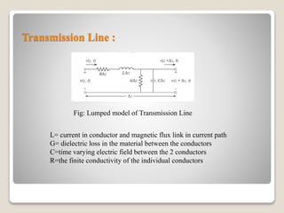
The document discusses microwave and radar engineering, focusing on transmission lines and waveguides, including their parameters and field solutions. It covers the design and analysis of rectangular and circular waveguides for TE10 and TE11 modes, respectively, providing key equations and learning outcomes. The pedagogical approach includes videos and detailed explanations of derivations relevant to the topic.

1. Presented by:
Anni Priyanka
Microwave and
Radar
Engineering

2. Objectives:
 R,L,C, G parameters of a co-axial & 2-wire transmission line
 Field solutions for TE and TM modes for a waveguide
 Design and analysis of rectangular waveguide to support TE10
mode
 Design and analysis of circular waveguide to support TE11
mode

3. Learning Outcome:
 Why transmission line uses lumped element model
 To calculate the TE wave equations in a rectangular wave
 To get the dominant mode in TE mode in a rectangular
waveguide

4. Novelty in pedagogy :
 The videos of concerned topic is presented
 Derivations are explained

5. Transmission Line :
L= current in conductor and magnetic flux link in current path
G= dielectric loss in the material between the conductors
C=time varying electric field between the 2 conductors
R=the finite conductivity of the individual conductors
Fig: Lumped model of Transmission Line

6. R,L,C, G parameters of a co-axial & 2-wire transmission line

7. Transmission line Vs. Waveguide :
Transmission Line Waveguide
It consists of two or more
conductors may support TEM waves
It consists of a single conductor,
support TE and/or TM waves
characterized by the lack of
longitudinal field components
It is characterized by the presence of
longitudinal magnetic or electric
field components
high power-handling capability, low
loss, but bulky and expensive
high bandwidth, convenient for test
applications, difficult medium in
which to fabricate complex
microwave components

8. General Solutions for TEM, TE and TM waves:
 General solutions to Maxwell’s equations for the specific cases of TEM, TE and
TM wave propagation in cylindrical transmission lines or waveguides.
 Uniform in z direction and infinitely long
Fig: (a)2-conductor transmission line (b)closed waveguide

9. E j H
H j E


  
 
Assume source free,
Proceeding from Maxwell curl equations,
,
,
z
y x
z
x y
y x
z
E
j E j H
y
E
j E j H
x
E E
j H
x y
 
 


  


   

 
  
 
,
,
z
y x
z
x y
y x
z
H
j H j E
y
H
j H j E
x
H H
j E
x y
 
 


 


  

 
  
 

10. By Solving these equations we will get:
2
2
z z
x
c
z z
y
c
j E H
H
k y x
j E H
H
k x y
 
 
  
  
  
   
  
  
2
2
z z
x
c
z z
y
c
j E H
E
k x y
j E H
E
k y x
 
 
   
  
  
  
   
  
As, 2 2 2
ck k  
Where, k is the wavenumber of the material filling with the
transmission line or waveguide region.
2 /k     
where kc: cutoff wavenumber,

11. For TE Waves:
Characterized by Ez = 0, Hz ≠ 0.
2
2
z
x
c
z
y
c
j H
H
k x
j H
H
k y


 


 


2
2
z
x
c
z
y
c
j H
E
k y
j H
E
k x


 





yx
TE
y x
EE k
Z
H H
 
 

   Impedance:

12. For TM Waves:
Characterized by Hz = 0, Ez ≠ 0
2
2
z
x
c
z
y
c
j E
H
k y
j E
H
k x





 


2
2
z
x
c
z
y
c
j E
E
k x
j E
E
k x


 


 


yx
TM
y x
EE
Z
H H k
 


   Impedance:

13. Attenuation due to Dielectric Loss:
• Using the complex dielectric constant
• In practice, most dielectric materials have a very small loss
(tan δ <<1). Using the Taylor expansion,
for x << a
2 2 2
2 2 2 2
0 0 (1 tan )
c
d c c r
k k
j k k k j

       
 
      
1/22 2 2
2 2 1 1
1 1
2 2
x x x
a x a a a
a a a
      
                    
;

14. • So, it reduces to
• For TE or TM wave :
• For TEM line, kc = 0, k = β
2
2 2 2 2 2
2 2
2
tan
tan
2
tan
2
c c
c
jk
k k jk k k
k k
k
j

 



    

 
;
2
tan
2
d
k 



tan
2
d
k 
 

15. Design and analysis of rectangular waveguide to support TE10 mode:
Fig: Geometry of rectangular waveguide

16. TE Modes
• Ez = 0
• Hz must satisfy Helmholtz equation :
2 2
2
2 2
( , ) 0c zk h x y
x y
  
   
  
( , ) ( ) ( )zh x y X x Y y
2 2
2
2 2
1 1
0c
d X d Y
k
X dx Y dy
  
Can be solved by separation and variables method by letting
Substituting in Helmholtz equation

17.  We define separation constant kx and ky such that
2 2
2 2 2 2 2
2 2
0, 0,x y x y c
d X d Y
k X k Y k k k
dx dy
     
( , ) ( cos sin )( cos sin )z x x y yh x y A k x B k x C k y B k y  
( , ) 0 at 0,
( , ) 0 at 0,
x
y
e x y y b
e x y x a
 
 
• Boundary conditions
• The general solution for hz can then be written as

18. Using these equations
2
2
( cos sin )( sin cos )
( sin cos )( cos sin )
x y x x y y
c
y x x x y y
c
j
e k A k x B k x C k y D k y
k
j
e k A k x B k x C k y D k y
k



   

   
( , , ) cos cos j z
z mn
m x n y
H x y z A e
a b
  

We get D = 0, and ky = nπ/b,
B = 0 , and kx = mπ/a

19.  The transverse field components of TEmn mode
( , , ) cos cos j z
z mn
m x n y
H x y z A e
a b
  

2
2
2
2
cos sin ,
sin cos ,
sin cos ,
cos sin .
j z
x mn
c
j z
y mn
c
j z
x mn
c
j z
y mn
c
j n m x n y
E A e
k b a b
j m m x n y
E A e
k a a b
j m m x n y
H A e
k a a b
j n m x n y
H A e
k b a b




   
   
   
   









• The final solution of Hz:

20. 2 2
2 2 2
c
m n
k k k
a b
 

   
       
   
2 2
c
m n
k k
a b
    
     
   
is real when
2 2
1
2 2
c
cmn
k m n
f
a b
 
   
   
     
   
The mode with the lowest cutoff frequency is called the
dominant mode;
10
1
2
cf
a 


21.  For f < fc, all field components will decay exponentially 
cutoff or evanescent modes
 The wave impedance
 The guide wavelength (λ: the wavelength of a plane wave in
the filling medium)
yx
TE
y x
EE k
Z
H H



  
2 2
g
k
 
 

   1/pv
k
 


  

22.  For the TE10 mode
10
10
10
cos ,
sin ,
sin ,
0.
j z
z
j z
y
j z
x
x z y
x
H A e
a
j a x
E A e
a
j a x
H A e
a
E E H




 

 








  
2 2
/ , ( / )ck a k a    

23.  The power flow down the guide for the TE10 mode:
 Attenuation can occur because of dielectric loss or
conductor loss.
0 0 0 0
2 2
210
2 0 0
3 2
10
2
1 1
ˆRe Re
2 2
Re( ) | |
sin
2
Re( ) | |
4
a b a b
o y x
x y x y
a b
x y
P E H zdydx E H dydx
a A x
dydx
a
a b A
  

 

 
   
 
   


   
 
2
| |
2
s
l s
C
R
P J dl 

24.  The attenuation due to conductor loss for TE10 mode
2 2 3
3 2
10
2 3 2
3
2
2 2 2
(2 ) /
l s
c
s
P R a a
b
P a b
R
b a k Np m
a b k
 

  

 
 
    
 
 

25. Cylindrical Co-ordinate systemRectangular Co-ordinate

26. Design and analysis of circular waveguide to support TE11 mode
Geometry of a circular waveguide

27. Bessel equations:
Bessel functions are solutions to the differential equation,
where k2 is real and n is an integer. The two independent solutions to this
equation are called ordinary Bessel functions of the first and second kind, written
as Jn(kρ) and Yn(kρ), and so the general solution to (C.1) is
Where,

28. 2 2
2 2
,
,
z z z z
c c
z z z z
c c
j E H j E H
E E
k k
j E H j E H
H H
k k
 
 
 
 
     
 
 
     
        
      
      
       
      
      
2
2 2 2
,
2 2
nm c nm
nm c cnm
p k p
k k k f
a a

   
  
      
 
General Solutions:

29. For TE11 mode: dominant mode
 
 
 
 
2
2
cos sin ( )
sin cos ( )
sin cos ( )
cos sin ( )
j z
n c
c
j z
n c
c
j z
n c
c
j z
n c
c
j n
E A n B n J k e
k
j
E A n B n J k e
k
j
H A n B n J k e
k
j n
H A n B n J k e
k









  


  

  

  






 
 

 

 

30. The wave impedance
TE
E E k
Z
H H
 
 



  
Consider the dominant TE11 mode with an excitation such that B = 0
1
1 12
1 12
sin ( ) , 0
cos ( ) , sin ( )
sin ( ) , cos ( )
j z
z c z
j z j z
c c
c c
j z j z
c c
c c
H A J k e E
j n j
E A J k e E A n J k e
k k
j j n
H A J k e H A n J k e
k k

 
 
 
 
 
 
   

 
   


 
 
 

 
 
 

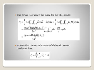
31. The power flow down the guide
2
0 0
2
0 0
2
2
2 2 2 2 2
1 14 20 0
2
2 2 2
1 14 20
1
ˆRe
2
1
Re [ ]
2
| | Re( ) 1
cos ( ) sin ( )
2
| | Re( ) 1
( ) ( )
2
| |
a
o
a
a
c c c
c
a
c c c
c
P E H z d d
E H E H dydx d d
A
J k k J k d d
k
A
J k k J k d
k
A

 

    

 

  
  
 
      

 
   



 
 
 
 

  
 
 
  
 
 
  
 

 
 
 

2
2 2
11 14
Re( )
( 1) ( )
4
c
c
p J k a
k

 

32. 4 2 2 2
2
2 2
11 11
( )
( )
2 ( 1) 1
l s c s
c c
o
P R k a R k
k
P k a p k a p


   

   
  
Attenuation constant:

33. Conclusion:
Derivation of equations for TE and TM modes in waveguides. And,
analysis of rectangular and cylindrical waveguide supporting the
dominant modes is done.

34. Review Questions:
 What is the use of waveguide?
 What are TM, TE and TEM waves?
 Why TEM mode cannot exist in the rectangular wave guide?
 Why is a dominant mode needed and how is it calculated?
 What are the uses of waveguide?

35. Semester Questions:
 Which mode in rectangular waveguide is dominant mode and why?
 Write the wave equations for a circular waveguide in a cylindrical coordinate
system?
 Why TE00 cannot exist in a rectangular waveguide?
 Write the field expression for TE10 mode of rectangular waveguide?
 Write the boundary conditions for the rectangular wave guide and circular wave
guide?
 Find out expression for power transmitted in a rectangular wave guide. Hence find
out expression of power delivered by TE10 mode?
 Find out expression for attenuation factor due to dielectric and conductivity in a
rectangular wave guide?
 Explain why TEM mode cannot exist in the rectangular wave guide?

36. References:
 David M. Pozar, "Microwave Engineering", Third Edition