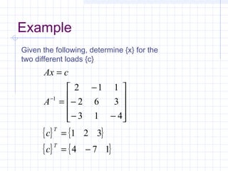
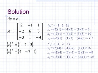
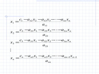
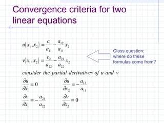
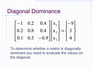
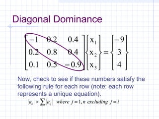
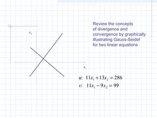
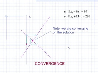
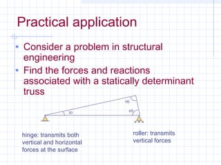
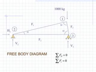
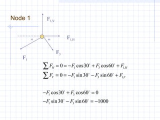
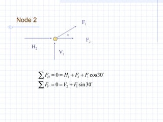
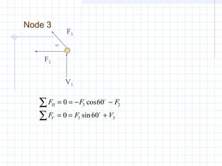
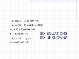
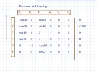
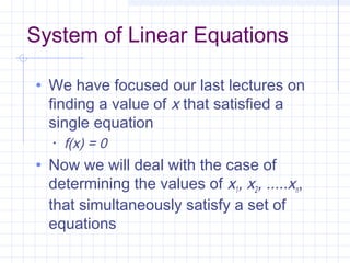
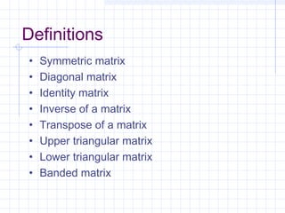
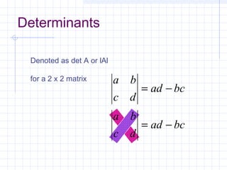
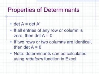
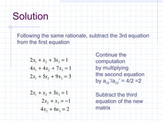
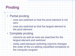
This document provides an overview of matrix methods for solving systems of linear equations. It begins with an example from structural engineering of setting up a system of 6 equations with 6 unknowns to model the forces and reactions in a statically determinant truss. The equations are represented in matrix notation as [A]{x}={c}. The document then reviews key matrix concepts and operations used to solve systems of linear equations, such as matrix addition, multiplication, transposes, inverses, and types of matrices. It aims to help readers understand how to set up and solve systems of linear equations using matrices.


![How to represent a system of linear
equations as a matrix
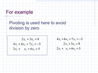
[A]{x} = {c}
where {x} and {c} are both column vectors](https://image.slidesharecdn.com/matrix-131010034223-phpapp01/85/Matrix-6-320.jpg)
![[ ]
−
−
=
=
−=++
=++
−=++
44.0
67.0
01.0
5.03.01.0
9.115.0
152.03.0
}{}{
44.05.03.01.0
67.09.15.0
01.052.03.0
3
2
1
321
321
321
x
x
x
CXA
xxx
xxx
xxx
How to represent a system of linear
equations as a matrix](https://image.slidesharecdn.com/matrix-131010034223-phpapp01/85/Matrix-7-320.jpg)
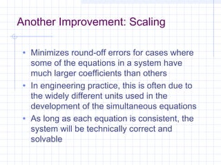
![This is the basis for your matrices and the equation
[A]{x}={c}
−
− −
− −
=
−
0866 0 05 0 0 0
05 0 0866 0 0 0
0 866 1 0 1 0 0
05 0 0 0 1 0
0 1 05 0 0 0
0 0 0866 0 0 1
0
1000
0
0
0
0
1
2
3
2
2
3
. .
. .
.
.
.
.
F
F
F
H
V
V](https://image.slidesharecdn.com/matrix-131010034223-phpapp01/85/Matrix-15-320.jpg)
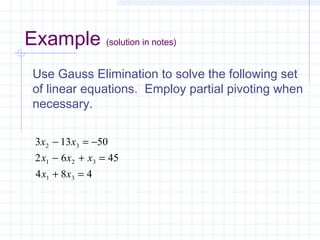
![Mathematical Background
Matrix Notation
• a horizontal set of elements is called a row
• a vertical set is called a column
• first subscript refers to the row number
• second subscript refers to column number
[ ]A
a a a a
a a a a
a a a a
n
n
m m m mn
=
11 12 13 1
21 22 23 2
1 2 3
...
...
. . . .
...](https://image.slidesharecdn.com/matrix-131010034223-phpapp01/85/Matrix-18-320.jpg)
![[ ]
=
mnmmm
n
n
aaaa
aaaa
aaaa
A
...
....
...
...
321
2232221
1131211
This matrix has m rows an n column.
It has the dimensions m by n (m x n)](https://image.slidesharecdn.com/matrix-131010034223-phpapp01/85/Matrix-19-320.jpg)
![[ ]
=
mnmmm
n
n
aaaa
aaaa
aaaa
A
...
....
...
...
321
2232221
1131211
This matrix has m rows and n column.
It has the dimensions m by n (m x n)
note
subscript](https://image.slidesharecdn.com/matrix-131010034223-phpapp01/85/Matrix-20-320.jpg)
![[ ]A
a a a a
a a a a
a a a a
n
n
m m m mn
=
11 12 13 1
21 22 23 2
1 2 3
...
...
. . . .
...
row 2
column 3
Note the consistent
scheme with subscripts
denoting row,column](https://image.slidesharecdn.com/matrix-131010034223-phpapp01/85/Matrix-21-320.jpg)
![Row vector: m=1
Column vector: n=1 Square matrix: m = n
[ ] [ ]B b b bn= 1 2 .......
[ ]C
c
c
cm
=
1
2
.
.
[ ]A
a a a
a a a
a a a
=
11 12 13
21 22 23
31 32 33
Types of Matrices](https://image.slidesharecdn.com/matrix-131010034223-phpapp01/85/Matrix-22-320.jpg)
![Symmetric Matrix
aij = aji for all i’s and j’s
[ ]A =
5 1 2
1 3 7
2 7 8
Does a23 = a32 ?
Yes. Check the other elements
on your own.](https://image.slidesharecdn.com/matrix-131010034223-phpapp01/85/Matrix-24-320.jpg)
![Diagonal Matrix
A square matrix where all elements
off the main diagonal are zero
[ ]A
a
a
a
a
=
11
22
33
44
0 0 0
0 0 0
0 0 0
0 0 0](https://image.slidesharecdn.com/matrix-131010034223-phpapp01/85/Matrix-25-320.jpg)
![Identity Matrix
A diagonal matrix where all elements
on the main diagonal are equal to 1
[ ]A =
1 0 0 0
0 1 0 0
0 0 1 0
0 0 0 1
The symbol [I] is used to denote the identify matrix.](https://image.slidesharecdn.com/matrix-131010034223-phpapp01/85/Matrix-26-320.jpg)
![Inverse of [A]
[ ][ ] [ ] [ ] [ ]IAAAA ==
−− 11](https://image.slidesharecdn.com/matrix-131010034223-phpapp01/85/Matrix-27-320.jpg)
![Transpose of [A]
[ ]A
a a a
a a a
a a a
t
m
m
n n mn
=
11 21 1
12 22 2
1 2
. . .
. . .
. . . . . .
. . . . . .
. . . . . .
. . .](https://image.slidesharecdn.com/matrix-131010034223-phpapp01/85/Matrix-28-320.jpg)
![Upper Triangle Matrix
Elements below the main diagonal
are zero
[ ]A
a a a
a a
a
=
11 12 13
22 23
33
0
0 0](https://image.slidesharecdn.com/matrix-131010034223-phpapp01/85/Matrix-29-320.jpg)
![Lower Triangular Matrix
All elements above the main
diagonal are zero
[ ]A =
5 0 0
1 3 0
2 7 8](https://image.slidesharecdn.com/matrix-131010034223-phpapp01/85/Matrix-30-320.jpg)
![Banded Matrix
All elements are zero with the
exception of a band centered on the
main diagonal
[ ]A
a a
a a a
a a a
a a
=
11 12
21 22 23
32 33 34
43 44
0 0
0
0
0 0](https://image.slidesharecdn.com/matrix-131010034223-phpapp01/85/Matrix-31-320.jpg)
![Matrix Operating Rules
• Addition/subtraction
• add/subtract corresponding terms
• aij + bij = cij
• Addition/subtraction are commutative
• [A] + [B] = [B] + [A]
• Addition/subtraction are associative
• [A] + ([B]+[C]) = ([A] +[B]) + [C]](https://image.slidesharecdn.com/matrix-131010034223-phpapp01/85/Matrix-32-320.jpg)
![Matrix Operating Rules
• Multiplication of a matrix [A] by a scalar
g is obtained by multiplying every
element of [A] by g
[ ] [ ]B g A
ga ga ga
ga ga ga
ga ga ga
n
n
m m mn
= =
11 12 1
21 22 2
1 2
. . .
. . .
. . . . . .
. . . . . .
. . . . . .
. . .](https://image.slidesharecdn.com/matrix-131010034223-phpapp01/85/Matrix-33-320.jpg)
![Matrix Operating Rules
• The product of two matrices is represented as
[C] = [A][B]
• n = column dimensions of [A]
• n = row dimensions of [B]
c a bij ik kj
k
N
=
=
∑1](https://image.slidesharecdn.com/matrix-131010034223-phpapp01/85/Matrix-34-320.jpg)
![[A] m x n [B] n x k = [C] m x k
interior dimensions
must be equal
exterior dimensions conform to dimension of resulting matrix
Simple way to check whether
matrix multiplication is possible](https://image.slidesharecdn.com/matrix-131010034223-phpapp01/85/Matrix-35-320.jpg)
![Recall the equation presented for
matrix multiplication
• The product of two matrices is represented as
[C] = [A][B]
• n = column dimensions of [A]
• n = row dimensions of [B]
c a bij ik kj
k
N
=
=
∑1](https://image.slidesharecdn.com/matrix-131010034223-phpapp01/85/Matrix-36-320.jpg)
![Example
Determine [C] given [A][B] = [C]
[ ]
[ ]
−
−
=
−
−
=
203
123
142
320
241
231
B
A](https://image.slidesharecdn.com/matrix-131010034223-phpapp01/85/Matrix-37-320.jpg)
![Matrix multiplication
• If the dimensions are suitable, matrix
multiplication is associative
• ([A][B])[C] = [A]([B][C])
• If the dimensions are suitable, matrix
multiplication is distributive
• ([A] + [B])[C] = [A][C] + [B][C]
• Multiplication is generally not
commutative
• [A][B] is not equal to [B][A]](https://image.slidesharecdn.com/matrix-131010034223-phpapp01/85/Matrix-38-320.jpg)
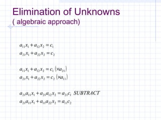
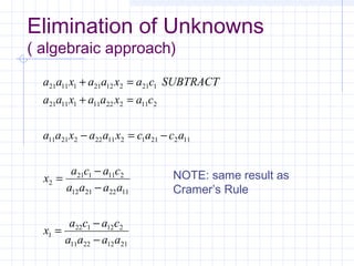
![Matrix Methods
• Cramer’s Rule
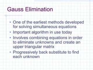
• Gauss elimination
• Matrix inversion
• Gauss Seidel/Jacobi
[ ]A
a a a
a a a
a a a
=
11 12 13
21 22 23
31 32 33](https://image.slidesharecdn.com/matrix-131010034223-phpapp01/85/Matrix-44-320.jpg)
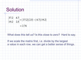
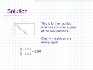
![Another Check
• Scale the matrix of coefficients, [A], so that the
largest element in each row is 1. If there are
elements of [A]-1
that are several orders of magnitude
greater than one, it is likely that the system is ill-
conditioned.
• Multiply the inverse by the original coefficient matrix.
If the results are not close to the identity matrix, the
system is ill-conditioned.
• Invert the inverted matrix. If it is not close to the
original coefficient matrix, the system is ill-
conditioned.
We will consider how to obtain an inverted matrix later.](https://image.slidesharecdn.com/matrix-131010034223-phpapp01/85/Matrix-57-320.jpg)
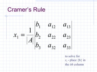
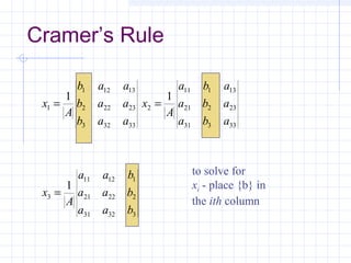
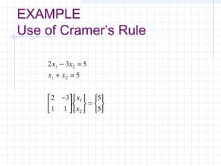
![Cramer’s Rule
• Not efficient for solving large numbers
of linear equations
• Useful for explaining some inherent
problems associated with solving linear
equations.
[ ]{ } { }bxA
b
b
b
x
x
x
aaa
aaa
aaa
=
=
3
2
1
3
2
1
333231
232221
131211](https://image.slidesharecdn.com/matrix-131010034223-phpapp01/85/Matrix-58-320.jpg)
![( )( ) ( )( )
( )( ) ( )( )[ ]
( )( ) ( )( )[ ]
2 3
1 1
5
5
2 1 3 1 2 3 5
1
5
5 3
5 1
1
5
5 1 3 5
20
5
4
1
5
2 5
1 5
1
5
2 5 5 1
5
5
1
1
2
1
2
−
=
= − − = + =
=
−
=
− − = =
= =
− = =
x
x
A
x
x
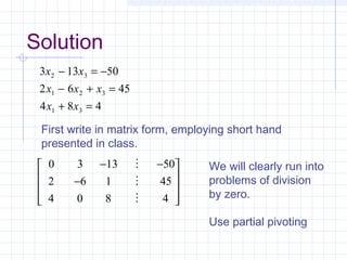
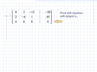
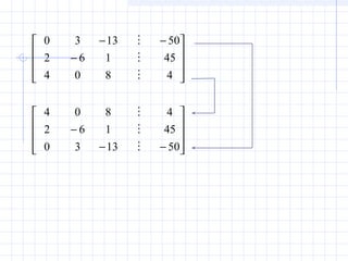
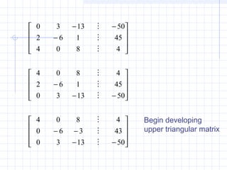
Solution](https://image.slidesharecdn.com/matrix-131010034223-phpapp01/85/Matrix-62-320.jpg)
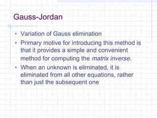
![• All rows are normalized by dividing them by
their pivot elements
• Elimination step results in an identity matrix
rather than an UT matrix
[ ]A
a a a
a a
a
=
11 12 13
22 23
33
0
0 0 [ ]A =
1 0 0 0
0 1 0 0
0 0 1 0
0 0 0 1
Gauss-Jordan](https://image.slidesharecdn.com/matrix-131010034223-phpapp01/85/Matrix-92-320.jpg)

![Matrix Inversion
• [A] [A] -1
= [A]-1
[A] = I
• One application of the inverse is to solve
several systems differing only by {c}
• [A]{x} = {c}
• [A]-1
[A] {x} = [A]-1
{c}
• [I]{x}={x}= [A]-1
{c}
• One quick method to compute the inverse is
to augment [A] with [I] instead of {c}](https://image.slidesharecdn.com/matrix-131010034223-phpapp01/85/Matrix-95-320.jpg)
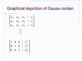
![Graphical Depiction of the Gauss-Jordan
Method with Matrix Inversion
[ ] [ ]
[ ] [ ]
A I
a a a
a a a
a a a
a a a
a a a
a a a
I A
11 12 13
21 22 23
31 32 33
11
1
12
1
13
1
21
1
22
1
23
1
31
1
32
1
33
1
1
1 0 0
0 1 0
0 0 1
1 0 0
0 1 0
0 0 1
− − −
− − −
− − −
−
Note: the superscript
“-1” denotes that
the original values
have been converted
to the matrix inverse,
not 1/aij](https://image.slidesharecdn.com/matrix-131010034223-phpapp01/85/Matrix-96-320.jpg)
![• [A]{x}={c}
• [interactions]{response}={stimuli}
• Superposition
• if a system subject to several different stimuli, the
response can be computed individually and the
results summed to obtain a total response
• Proportionality
• multiplying the stimuli by a quantity results in the
response to those stimuli being multiplied by the
same quantity
• These concepts are inherent in the scaling of terms
during the inversion of the matrix
Stimulus-Response Computations](https://image.slidesharecdn.com/matrix-131010034223-phpapp01/85/Matrix-99-320.jpg)