Downloaded 38 times

![Simulation: Covariate generating model
Based on Franklin et al. Metrics for covariate balance in cohort
studies of causal effects. Stat Med. 2014;33:1685.
Variable Generation Process
X1i Normal(0, 12
)
X2i Log-Normal(0, 0.52
)
X3i Normal(0, 102
)
X4i Bernoulli(pi = e2X1i
/(1 + e2X1i
)) where E[pi ] = 0.5
X5i Bernoulli(p = 0.2)
X6i Multinomial(p = (0.5, 0.3, 0.1, 0.05, 0.05)T
)
X7i sin(X1i )
X8i X2
2i
X9i X3i × X4i
X10i X4i × X5i
17 / 31](https://image.slidesharecdn.com/slides-160712192546/75/Matching-Weights-to-Simultaneously-Compare-Three-Treatment-Groups-a-Simulation-Study-17-2048.jpg)

![Empirical example: Outcome regression
Yoshida K et al. Matching Weights for Three-category Exposure 2/9/2016
Table 1. Comparison of hazard ratios for coxibs and opioids (nonselective NSAIDs as the reference)
by different methods and outcomes.
Coxibs vs nsNSAIDs Opioids vs nsNSAIDs
HR [95% CI] p HR [95% CI] p
Death
Unmatched 1.702 [1.293, 2.240] <0.001 2.821 [2.185, 3.642] <0.001
Matched 1.415 [1.060, 1.889] 0.018 1.997 [1.492, 2.671] <0.001
MW 1.393 [1.056, 1.837] 0.019 1.973 [1.517, 2.566] <0.001
IPTW 1.385 [1.024, 1.873] 0.035 1.962 [1.480, 2.601] <0.001
Fracture
Unmatched 1.181 [0.799, 1.746] 0.405 5.825 [4.195, 8.089] <0.001
Matched 0.947 [0.618, 1.453] 0.804 4.708 [3.308, 6.702] <0.001
MW 1.013 [0.684, 1.502] 0.948 4.733 [3.396, 6.595] <0.001
IPTW 0.887 [0.576, 1.365] 0.585 4.068 [2.814, 5.882] <0.001
GI bleed
Unmatched 0.933 [0.605, 1.439] 0.753 1.529 [1.034, 2.262] 0.033
Matched 0.932 [0.587, 1.480] 0.766 1.005 [0.615, 1.643] 0.984
MW 0.857 [0.551, 1.335] 0.496 1.108 [0.737, 1.668] 0.622
IPTW 0.916 [0.575, 1.459] 0.713 1.196 [0.793, 1.804] 0.394
Cardiovascular
Unmatched 1.603 [1.298, 1.979] <0.001 2.294 [1.882, 2.797] <0.001
Matched 1.419 [1.135, 1.775] 0.002 1.585 [1.255, 2.003] <0.001
MW 1.355 [1.096, 1.675] 0.005 1.626 [1.326, 1.995] <0.001
IPTW 1.268 [0.979, 1.642] 0.072 1.445 [1.125, 1.856] 0.004 30 / 31](https://image.slidesharecdn.com/slides-160712192546/75/Matching-Weights-to-Simultaneously-Compare-Three-Treatment-Groups-a-Simulation-Study-30-2048.jpg)
![Outline of proof that estimands are equivalent
A complete common support and exact propensity score matching are
assumed. Sk is the set of matched individuals in treatment group k. Wi
is the matching weights min(e1i ,...,eKi )
K
k=1 I(Zi =k)eki
. The estimators for the group
mean have the same estimand.
Matching
1
n
n
i=1 Yi I(i ∈ Sk )
1
n
n
i=1 I(i ∈ Sk )
=
1
n
n
i=1 Yki I(i ∈ Sk )
1
n
n
i=1 I(i ∈ Sk )
→
E[Yki I(i ∈ Sk )]
E[I(i ∈ Sk )]
. . .
=
E [E[Yki |Xi ]min(e1i , ..., eKi )]
E [min(e1i , ..., eKi )]
Weighting
1
n
n
i=1 Yi I(Zi = k)Wi
1
n
n
i=1 I(Zi = k)Wi
=
1
n
n
i=1 Yki I(Zi = k)Wi
1
n
n
i=1 I(Zi = k)Wi
→
E[
n
i=1 Yki I(Zi = k)Wi ]
E[
n
i=1 I(Zi = k)Wi ]
. . .
=
E [E[Yki |Xi ]min(e1i , ..., eKi )]
E [min(e1i , ..., eKi )] 31 / 31](https://image.slidesharecdn.com/slides-160712192546/75/Matching-Weights-to-Simultaneously-Compare-Three-Treatment-Groups-a-Simulation-Study-31-2048.jpg)

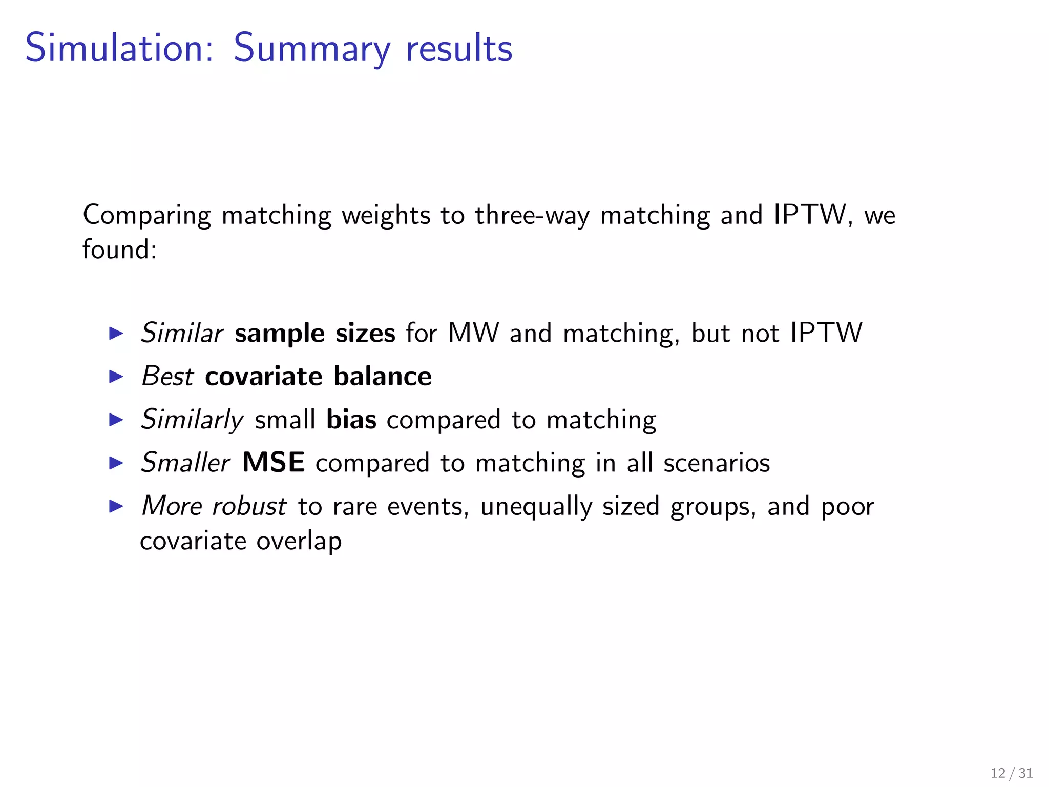
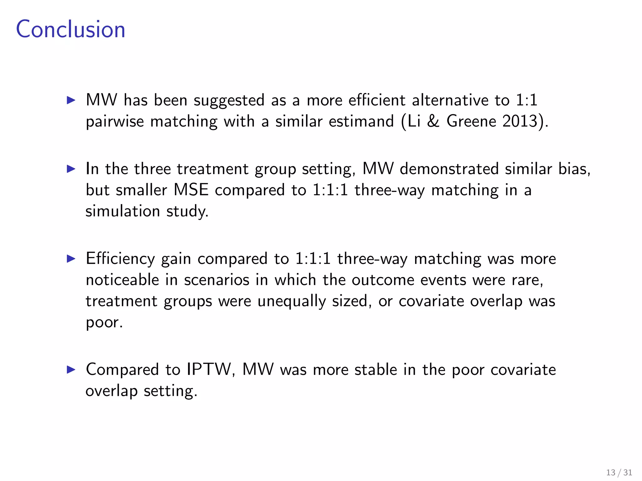
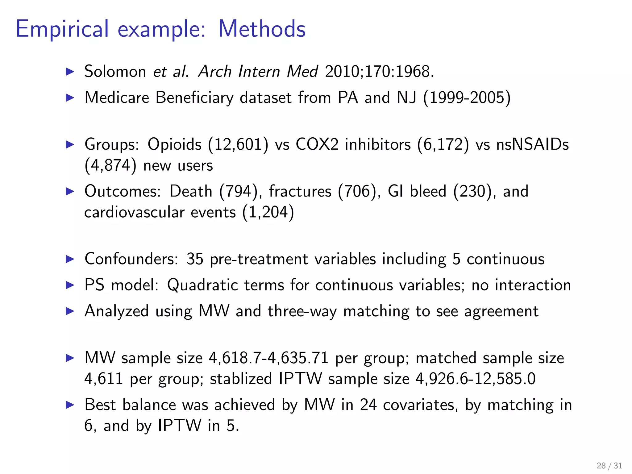
This document discusses a simulation study comparing matching weights to three-way matching and inverse probability treatment weighting (IPTW) in clinical settings with three or more treatment groups. The findings suggest that matching weights offer an efficient alternative, providing similar bias but smaller mean squared error (MSE) compared to traditional methods, particularly in scenarios with rare outcomes and poor covariate overlap. Ultimately, matching weights may be more robust for non-binary treatment comparisons in clinical research.
Presentation introduces matching weights for treatment comparison in clinical studies.
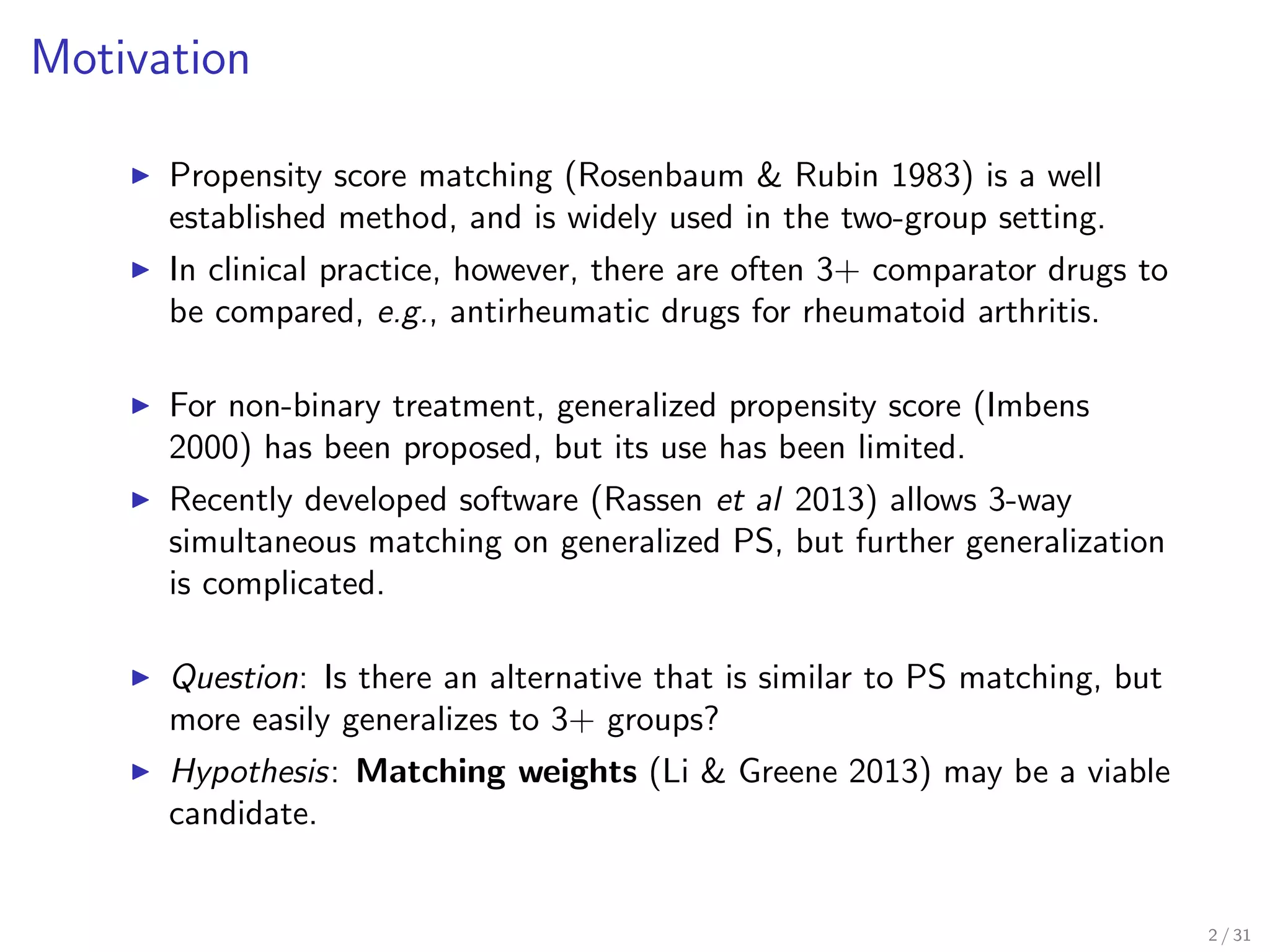
Highlights the limitations of existing propensity score methods in comparing multiple treatments.
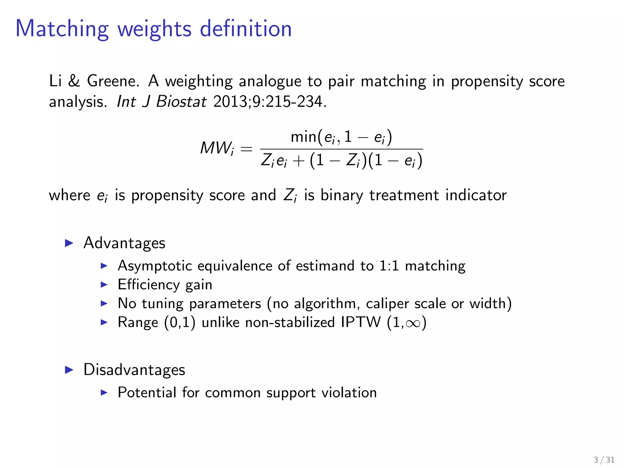
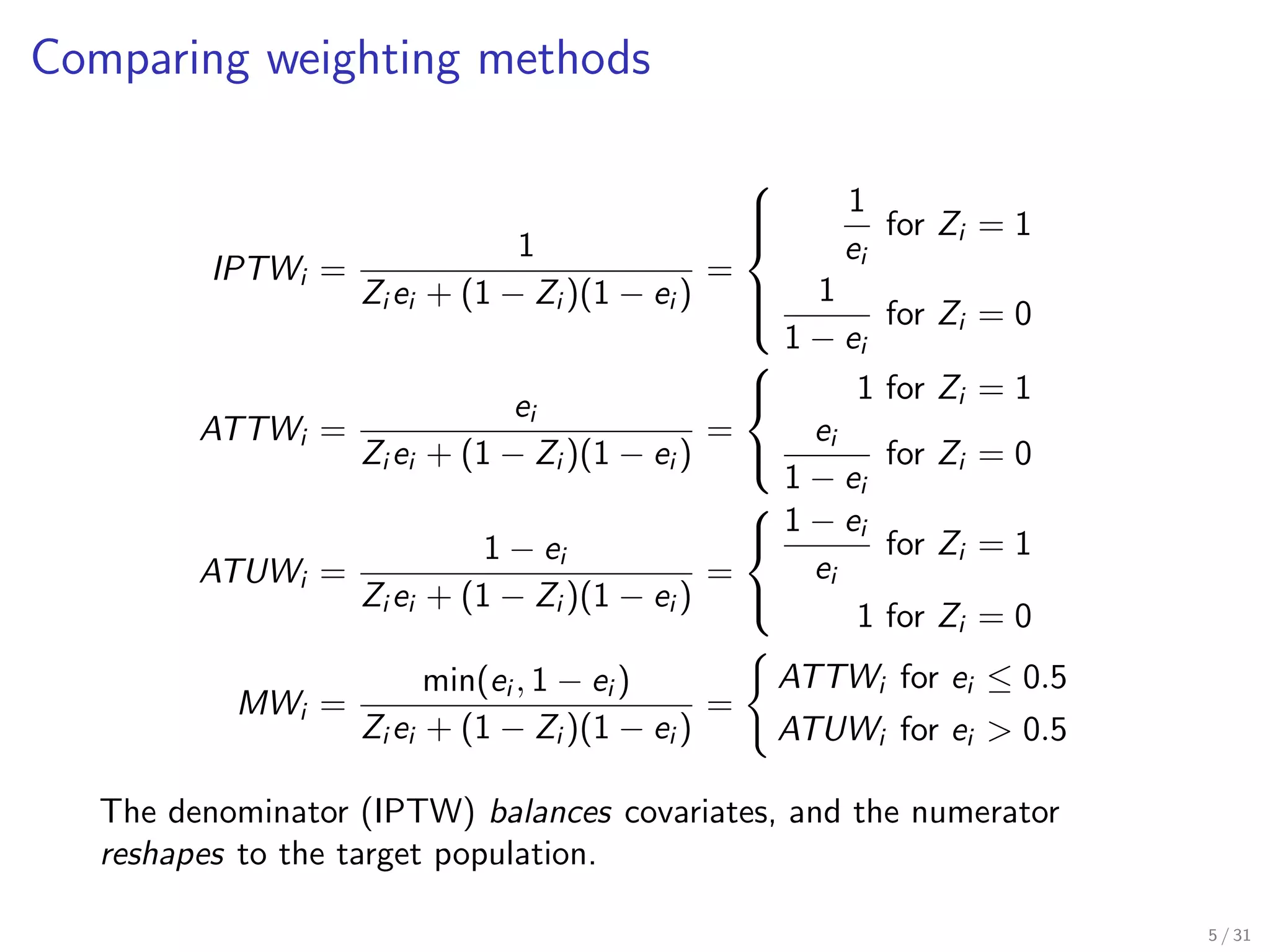
Details the formula for matching weights and discusses advantages and disadvantages.
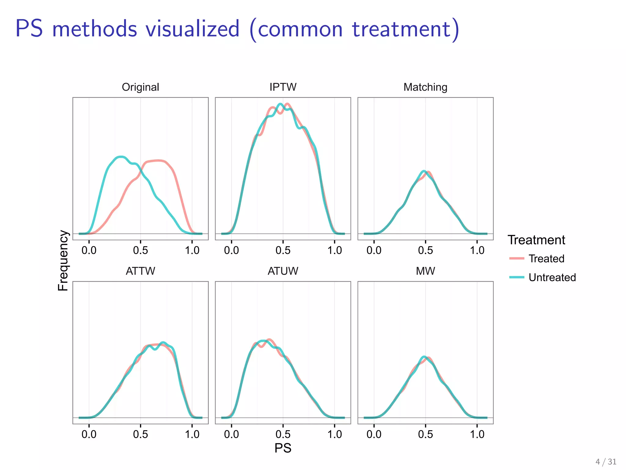
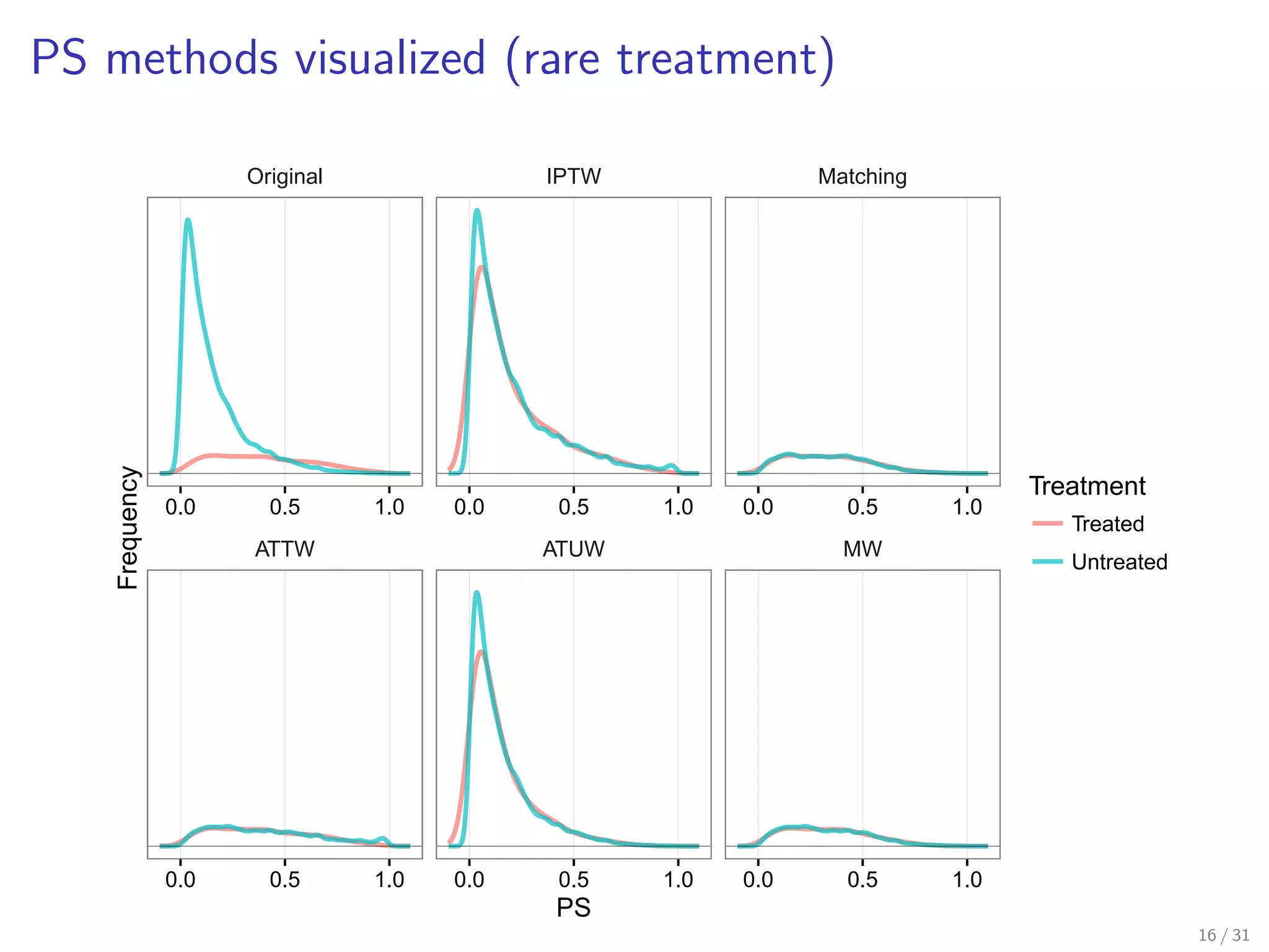
Illustrates treatment distributions for different propensity score methods.
Summarizes various weighting methods and their computational representations.
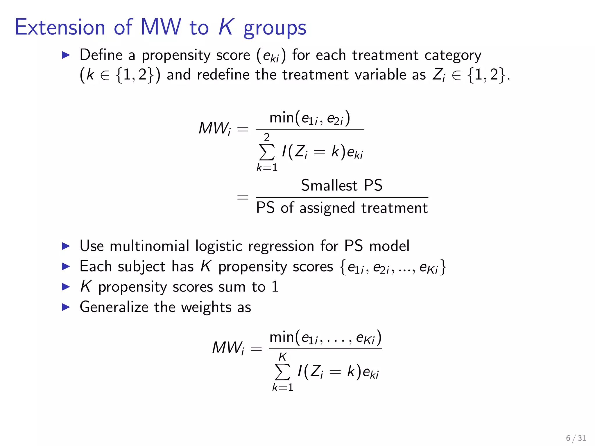
Explains how to adapt matching weights for K treatment groups using new definitions.
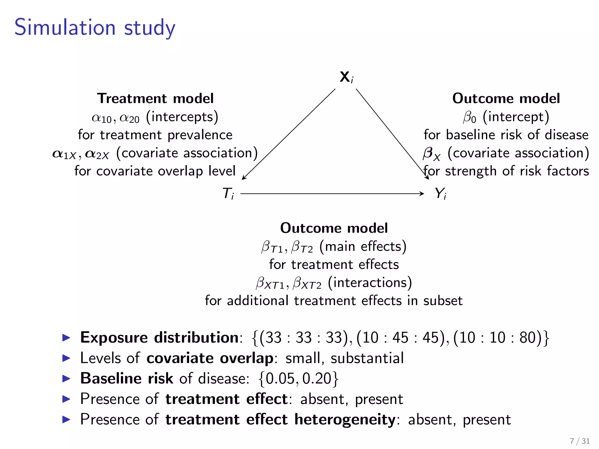
Outlines the simulation study framework for evaluating treatment effects and covariate overlap.
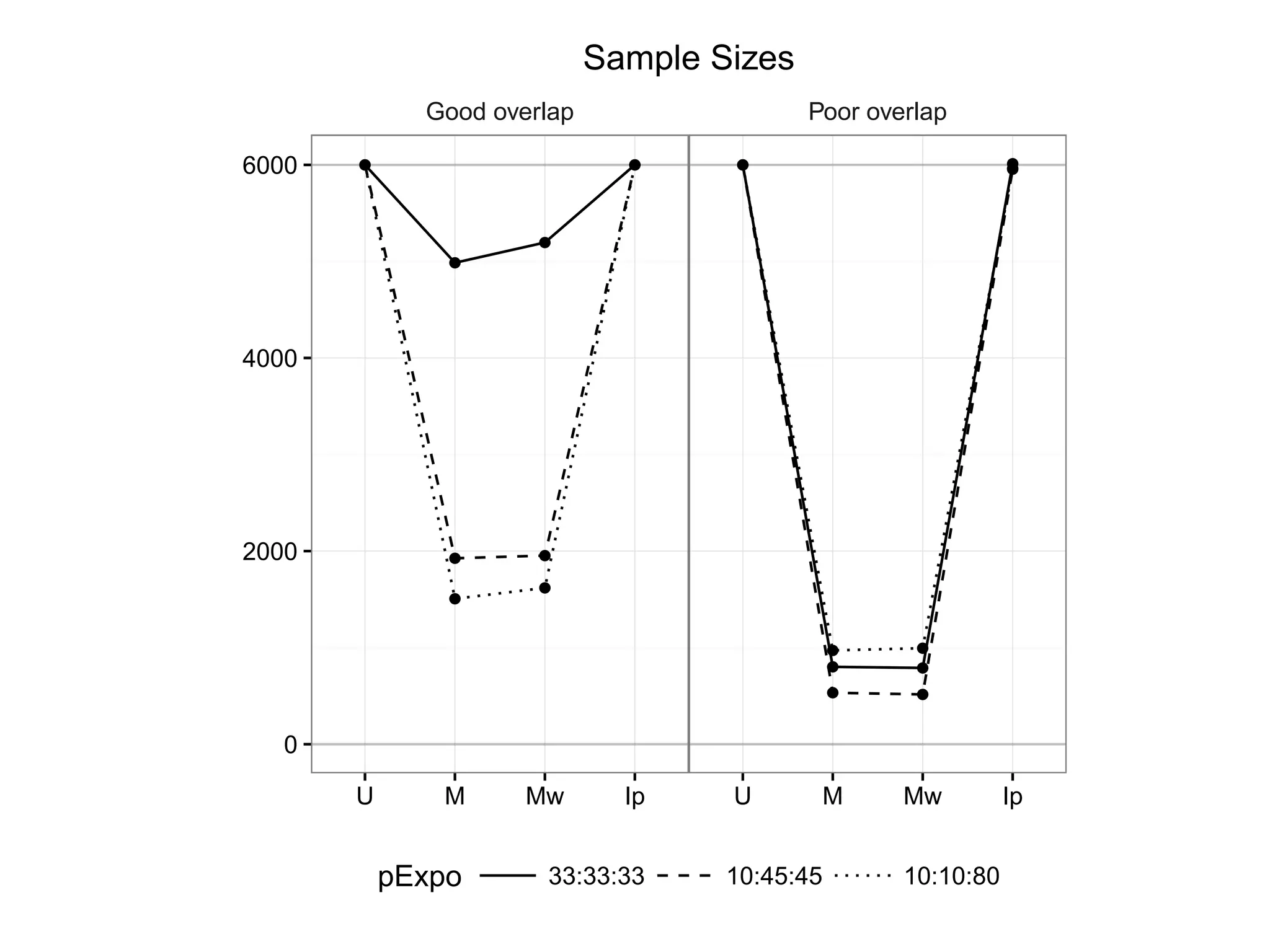
Presents outcomes comparing performance under good and poor overlap scenarios.
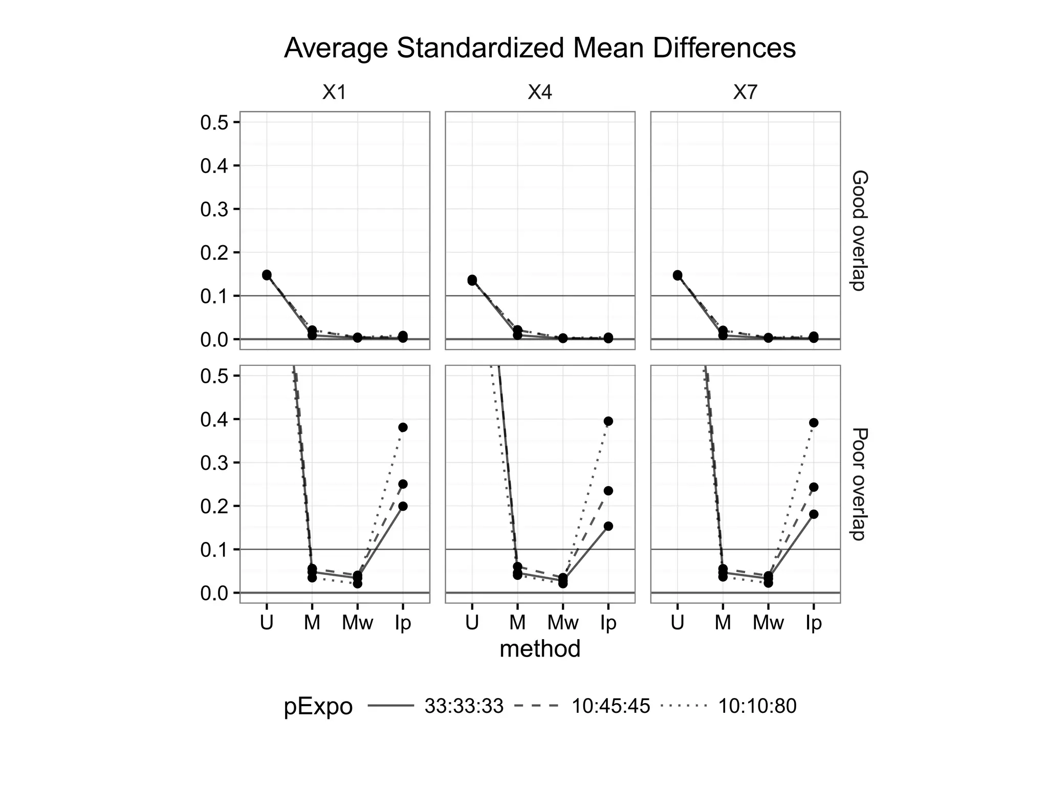
Examines standardized mean differences in covariates across various treatment overlap conditions.
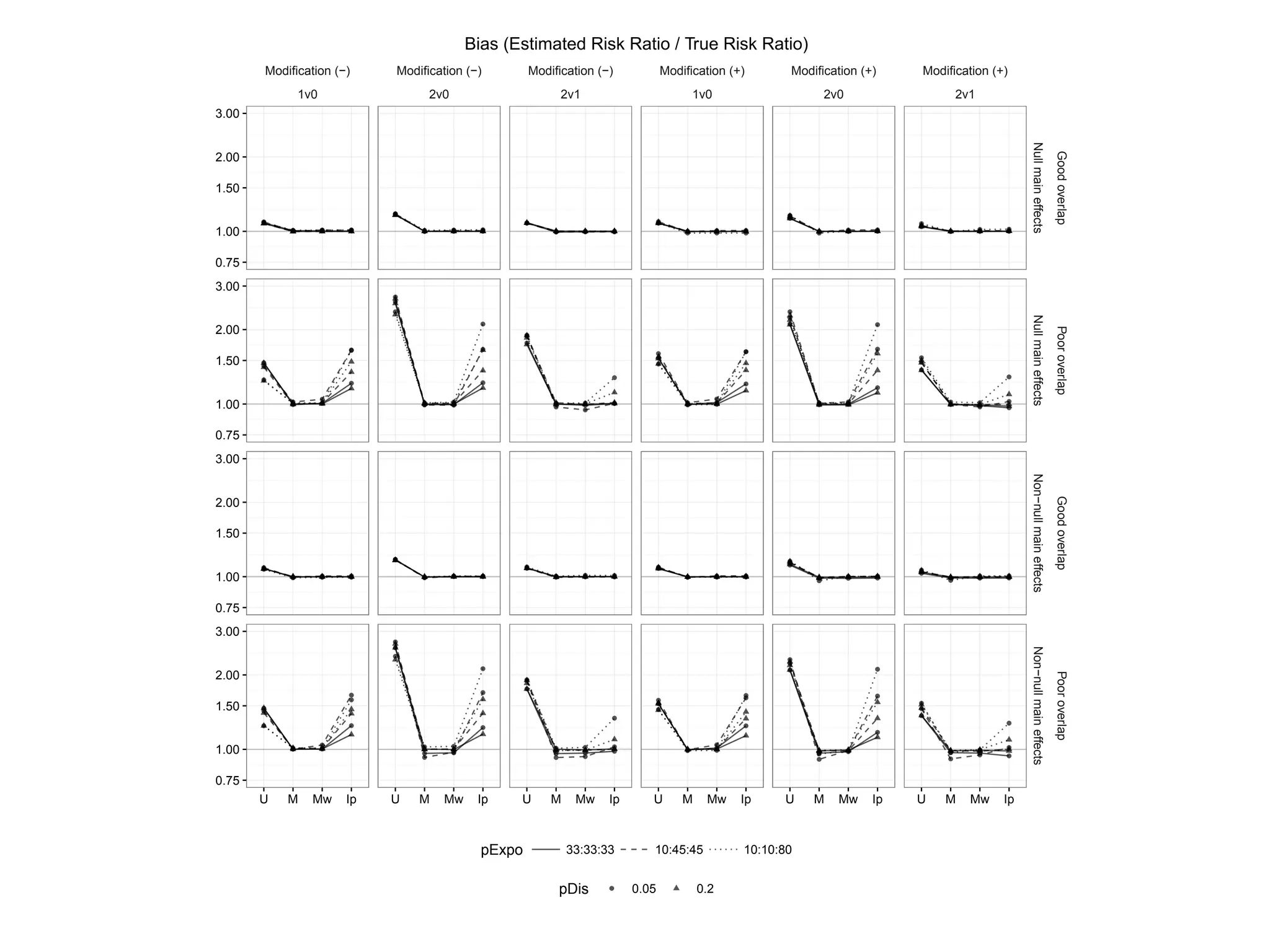
Analyzes bias in estimated risk ratios under different treatment modifications.
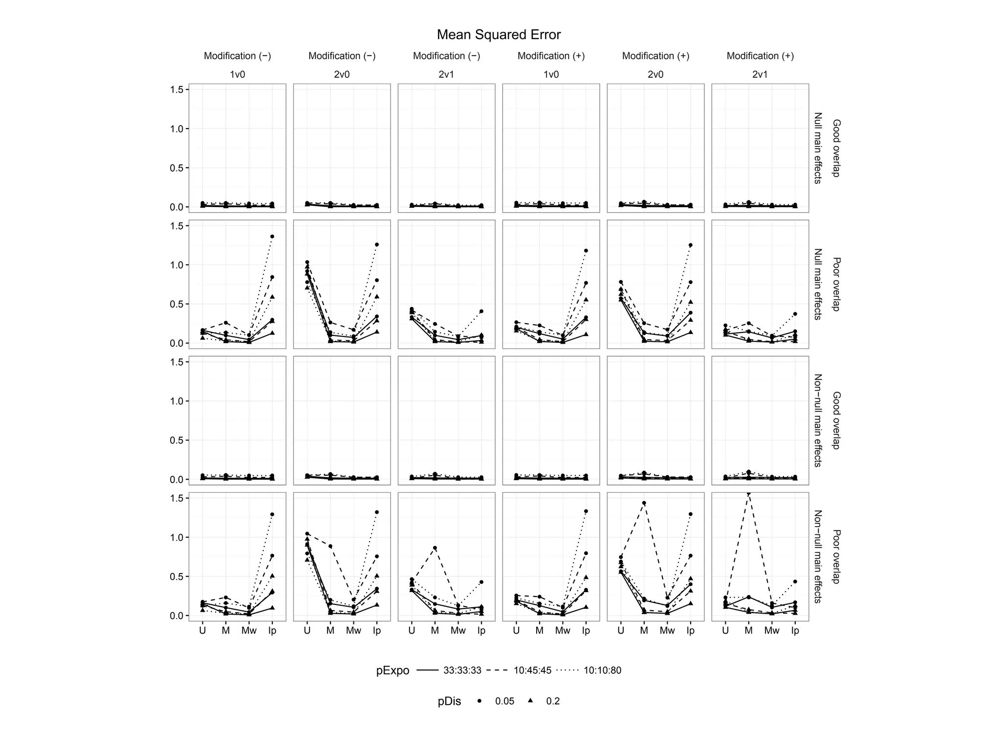
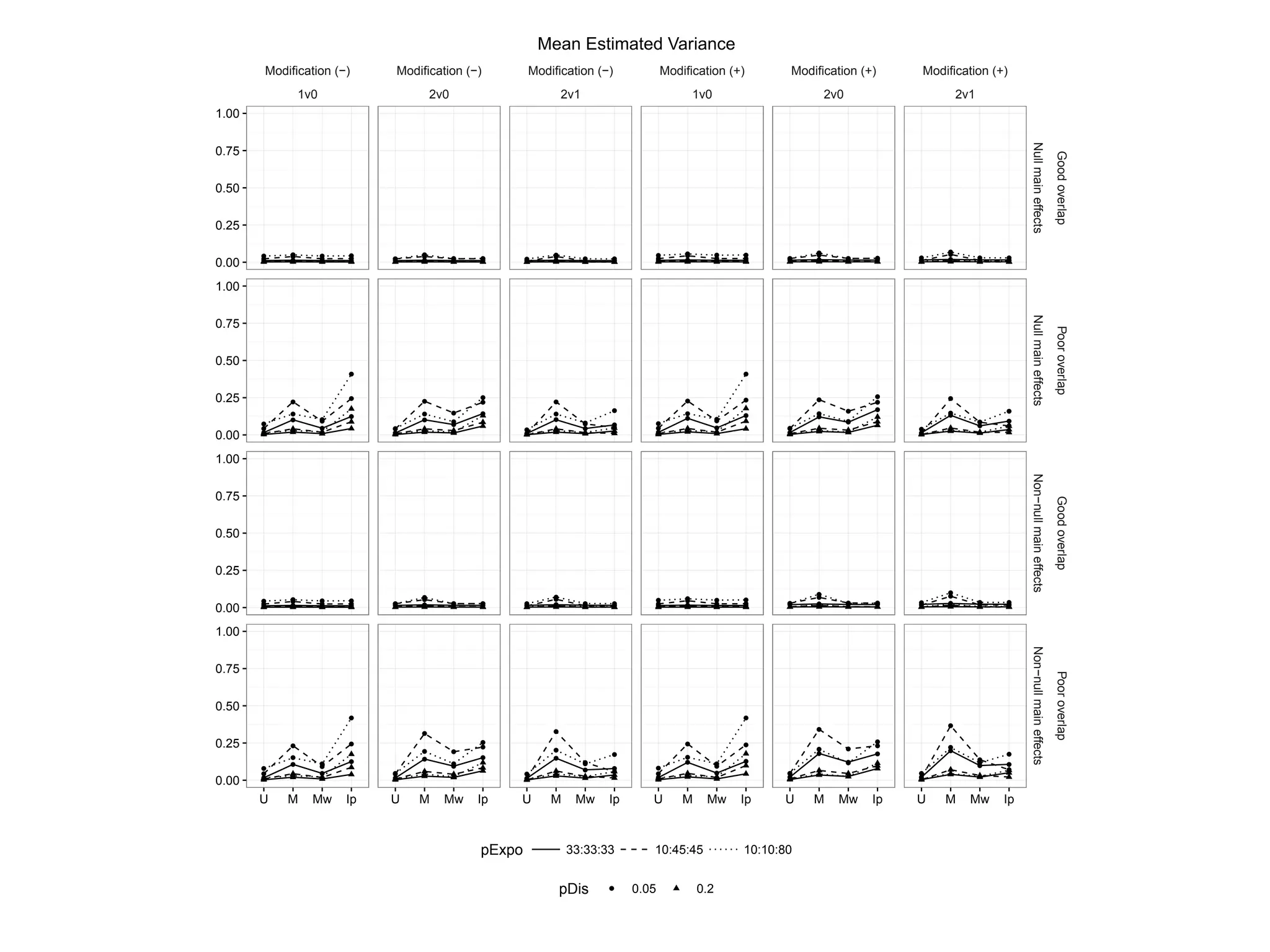
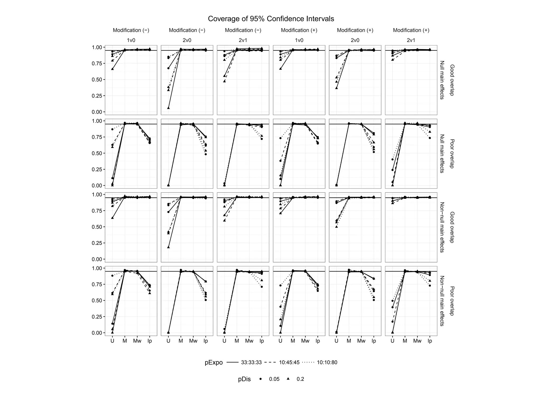
Evaluates simulation results through mean squared error across different treatment alignments.
Compares matching weights against three-way matching and IPTW in terms of bias and MSE.
Summarizes findings, recommending MW as a more efficient alternative in treatment comparisons.
Credits funding sources for the research conducted.
Announces forthcoming slides that delve into further details.
Similar visualization for rare treatment outcomes in propensity score methods.
Describes the model processes used for generating treatment covariates in simulations.
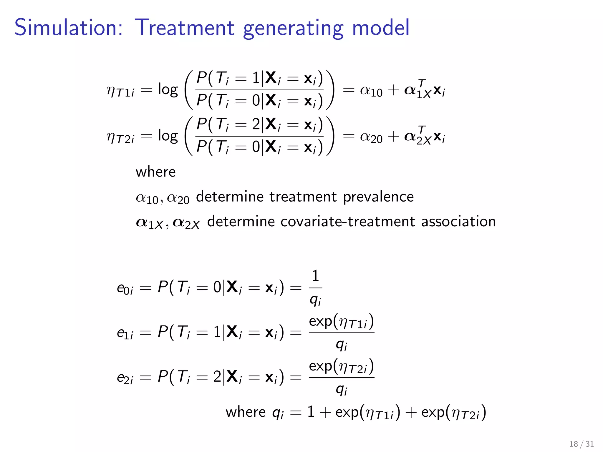
Details the model for determining treatment prevalence and covariate associations.
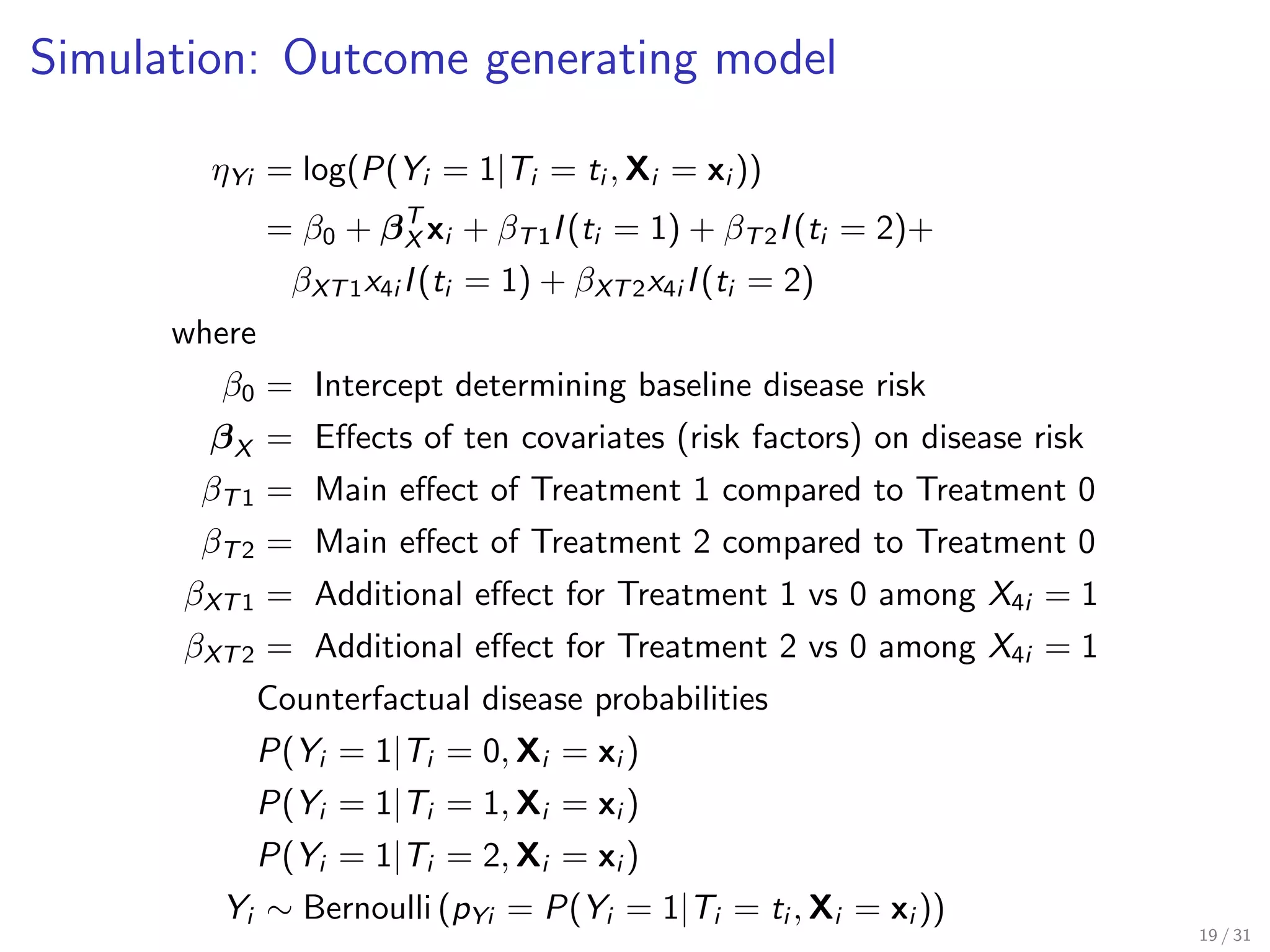
Explains the process for modeling treatment effects on disease outcomes.
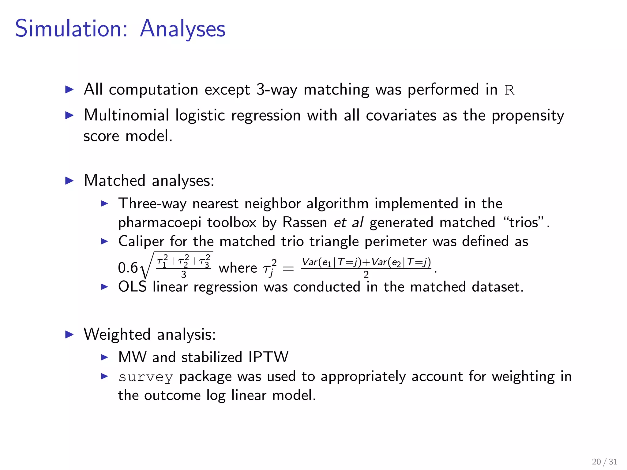
Describes analytical methods and computations used in simulation analysis.
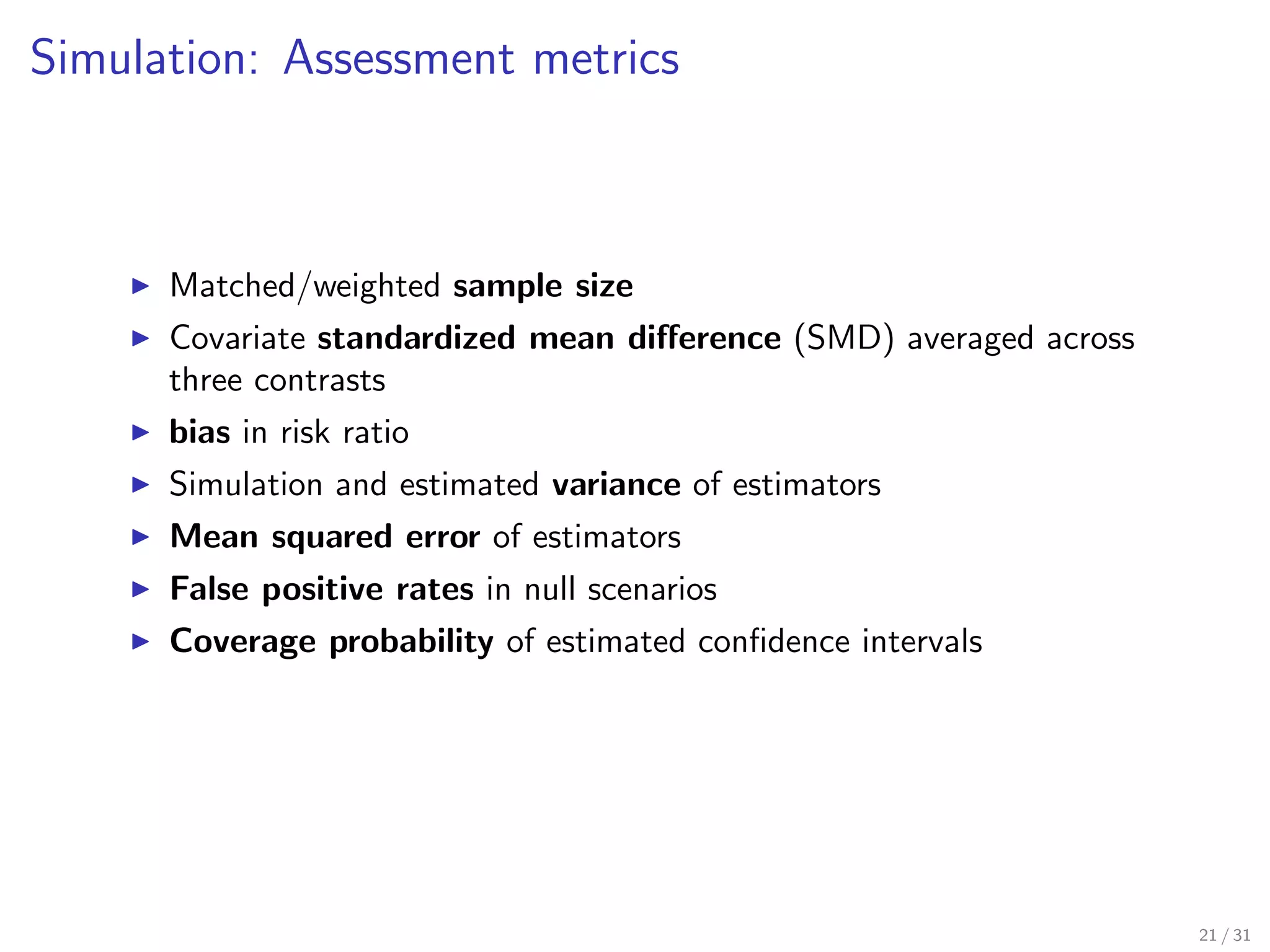
Lists metrics for evaluating the results of simulation analyses.
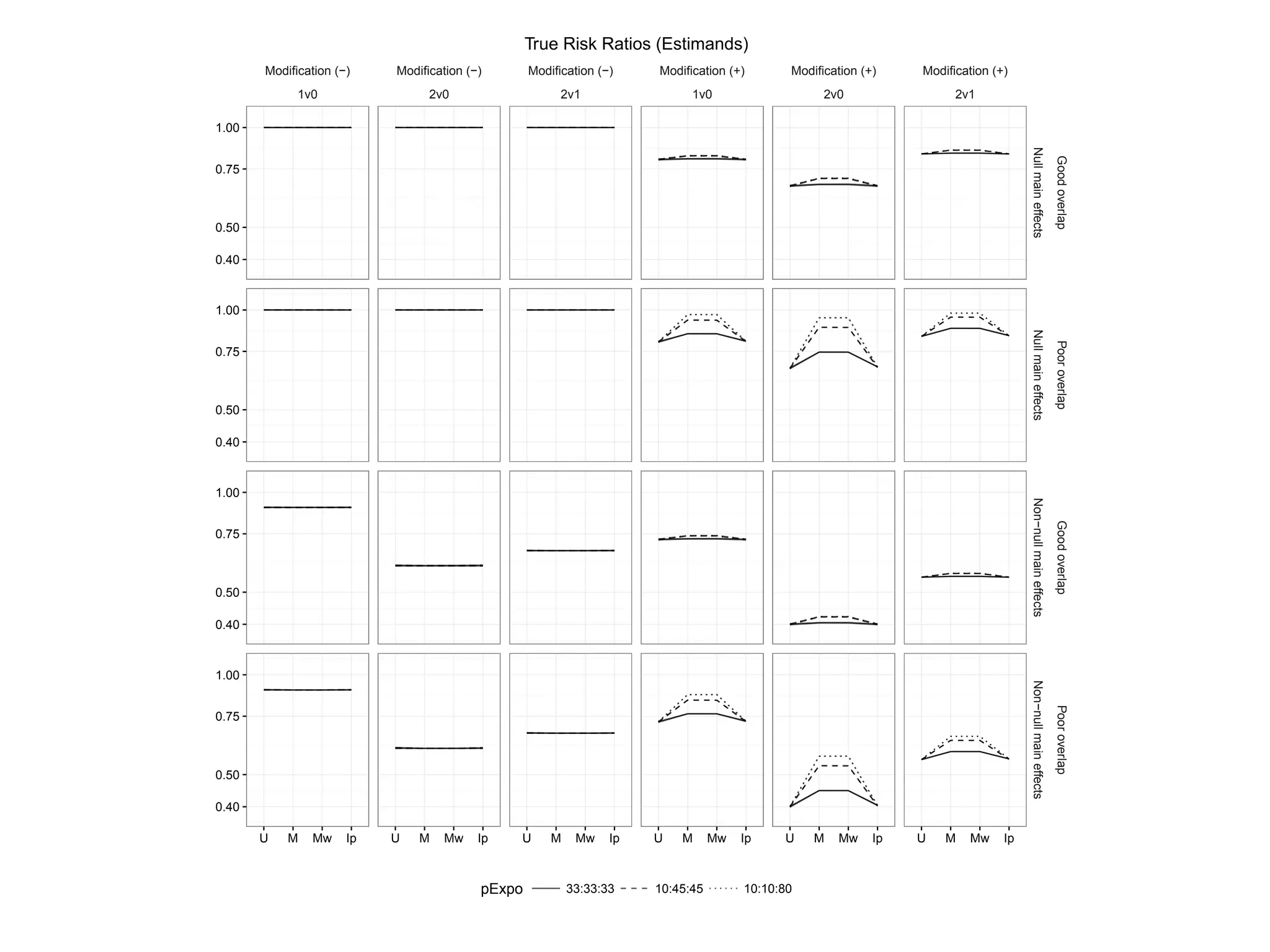
Shows the impact of various modifications on estimated treatment risk ratios.
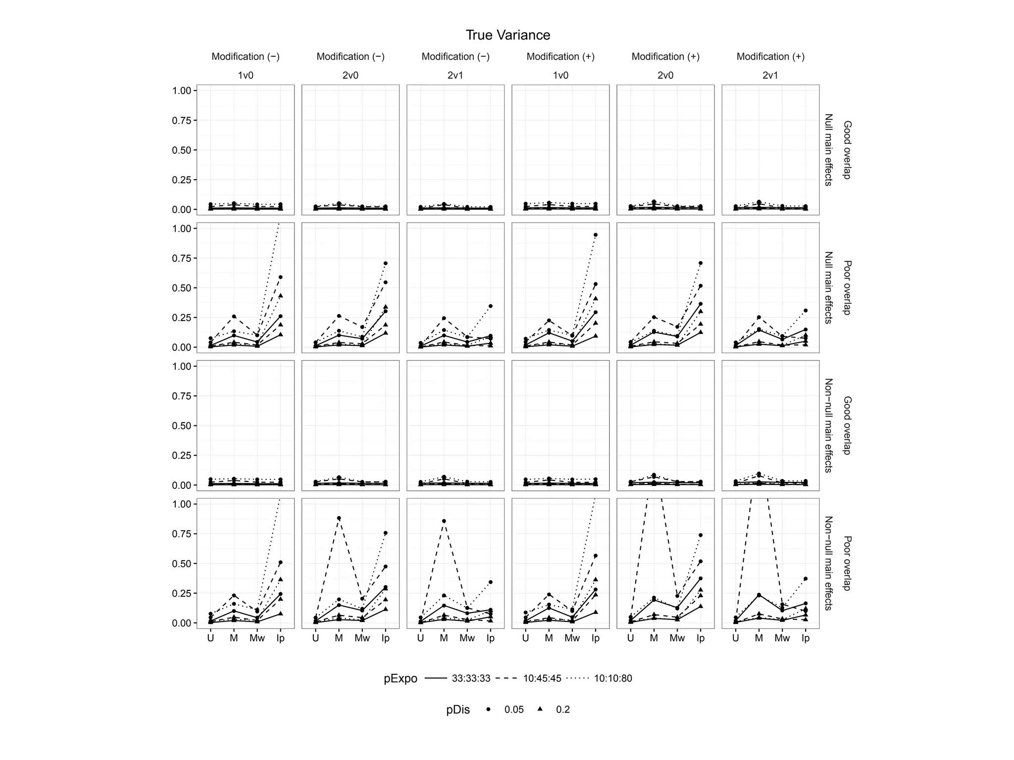
Analyzes variance to highlight changes in treatment effect estimates.
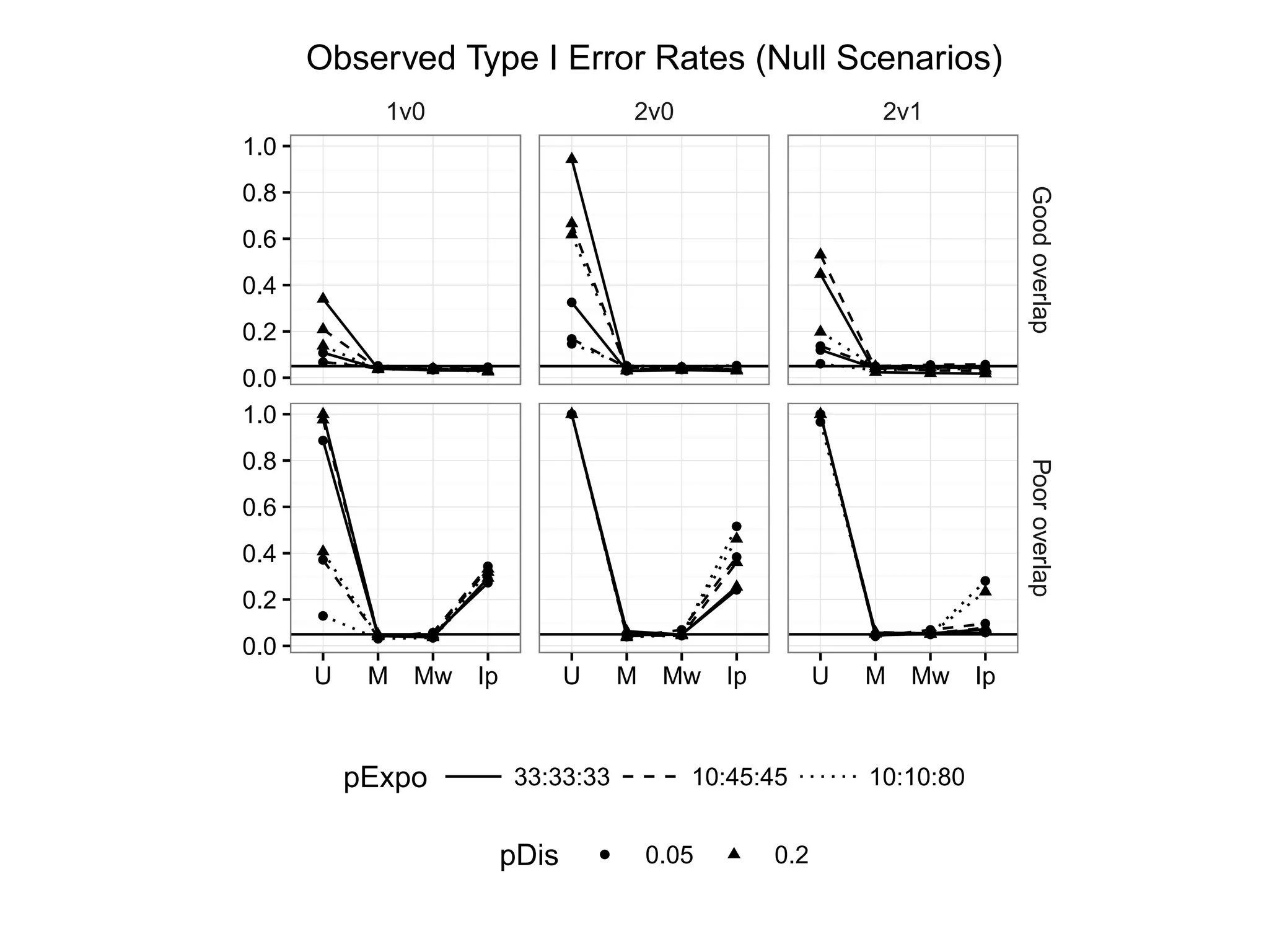
Evaluates the performance of methods across observed Type I error rates.
Describes an empirical application using Medicare data for analgesic comparisons.
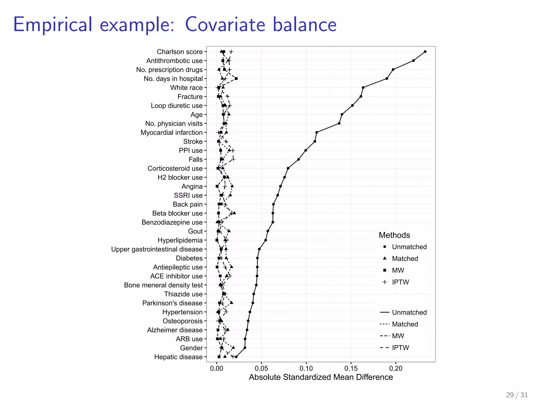
Reports on covariate balance achieved through different methods in treatment comparison.
Summarizes hazard ratios comparing outcomes between treatment groups.
Presents proof of equivalence between matching and weighting estimators.


![[DSC Europe 25] Marija Vlajkovic & Andrea Radonjanin - Integration of AI tool...](https://cdn.slidesharecdn.com/ss_thumbnails/qf1jrglttoc3bm8s3aop-final-integration-of-ai-tools-251208151905-394f3a6a-thumbnail.jpg?width=640&height=640&fit=bounds)

![[DSC Europe 25] Nikola Rajovic - Hardware Technologies Under the Hood: RISC-V...](https://cdn.slidesharecdn.com/ss_thumbnails/o2gptrmtoyqndgoshwgq-dsc2025-tenstorrent-rajovic-251205090438-814685f5-thumbnail.jpg?width=640&height=640&fit=bounds)
![[DSC Europe 25] Goran Obradovic - The Rise of Sovereign AI: Building the Regi...](https://cdn.slidesharecdn.com/ss_thumbnails/7nw2xxixrxqdxvrb5wca-6-251205085714-ab09a2ac-thumbnail.jpg?width=640&height=640&fit=bounds)


![[DSC Europe 25] Dragana Ilic - AI for Big Data in Astronomy.pptx](https://cdn.slidesharecdn.com/ss_thumbnails/8palya86qaatvjhva1ms-2-dragana-ilic-ai-ilic-251208151906-652b819c-thumbnail.jpg?width=640&height=640&fit=bounds)


![[DSC Europe 25] Bogdan Daniel Maruneac - AI - It starts with you.pptx](https://cdn.slidesharecdn.com/ss_thumbnails/odov3snhrcqs9hx5ny2n-4-251205085715-f1daacfe-thumbnail.jpg?width=640&height=640&fit=bounds)


![[DSC Europe 25] Boris Perkovic - Lost in performance.pptx](https://cdn.slidesharecdn.com/ss_thumbnails/uq5hrp7vsuahqkxzifux-1-251204082258-fd2ee09d-thumbnail.jpg?width=640&height=640&fit=bounds)

![[DSC Europe 25] Petar Zivanov - AI meets documents From chatbots to AI-powere...](https://cdn.slidesharecdn.com/ss_thumbnails/xer2bb6nrdc8pdpev0pc-8-251204082258-7c2fa4a1-thumbnail.jpg?width=640&height=640&fit=bounds)


