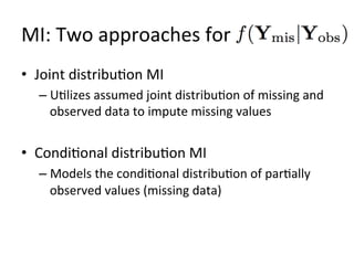
The document discusses multiple imputation (MI) as a method for addressing missing data in datasets, reviewing its algorithms, strengths, and weaknesses. It contrasts joint distribution MI and conditional distribution MI approaches, noting implications for high-dimensional data and the challenges faced with covariance matrices. The conclusion emphasizes that while the joint approach is theoretically sound, both methods struggle with high-dimensional cases where covariates exceed observations.

1. Mul$ple Imputa$on
Octavious Talbot & Kazuki Yoshida
Dec 16, 2015
BIO235 Final Project
This document was created by students to fulfill a course requirement. Be aware of
poten$al errors, and check with the original papers. There is a corresponding report
document at hPps://github.com/kaz-yos/misc/blob/master/MI_Project.Rnw.pdf

2. Outline
• Background
• Mul$ple Imputa$on
– Joint Distribu$on
– Condi$onal Distribu$on
• Compare/Contrast
• Conclusion

3. Background
• Missing data is an omnipresent problem that
affects almost all real datasets.
• MI has become one of the most popular
methods to address missing data.
• We review major MI algorithms, including
their rela$ve strengths and weaknesses and
implica$ons for high-dimensional data.

4. Missing data classifica$on
• Missing Completely At Random (MCAR)
• Missing At Random (MAR)
• Not Missing At Random (NMAR)

5. Approaches
• Insufficient
– Complete cases, indicator, single imputa$on

6. Approaches
• Insufficient
– Complete cases, indicator, single imputa$on
• BePer
– Mul$ple imputa$on

7. Approaches
• Insufficient
– Complete cases, indicator, single imputa$on
• BePer
– Mul$ple imputa$on
– Likelihood-based
– Weigh$ng

8. Approaches
• Insufficient
– Complete cases, indicator, single imputa$on
• BePer
– Mul$ple imputa$on
– Likelihood-based
– Weigh$ng
• Best

9. Approaches
• Insufficient
– Complete cases, indicator, single imputa$on
• BePer
– Mul$ple imputa$on
– Likelihood-based
– Weigh$ng
• Best
– Preven$on

10. Theory behind MI
• Posterior distribu$on of quan$ty of interest Q
given observed data only
• Likelihood-based approaches such as full
informa$on maximum likelihood (FIML) model
this expression itself. But it can be difficult.

11. Theory behind MI
• Posterior distribu$on of quan$ty of interest Q
given observed data only
• Decompose into more tractable parts.
– Distribu$on of Q given complete data (outcome
model)
– Distribu$on of missing data given observed data
(missing data model)
– Integra$on over missing data distribu$on

12. Overview of MI
van Buuren 1999
Rubin’s rule

13. Overview of MI
Impute based on
missing data model
Outcome model using
complete data
“Integrate” over
imputed datasets
What you get
LiPle 2002

14. MI: Two approaches for
• Joint distribu$on MI
– U$lizes assumed joint distribu$on of missing and
observed data to impute missing values
• Condi$onal distribu$on MI
– Models the condi$onal distribu$on of par$ally
observed values (missing data)

15. Joint approach
• Two main approaches
– Imputa$on-Posterior (IP) algorithm
– Expecta$on Maximiza$on (EM) algorithm
• Usual Assump$ons
– MVN joint distribu$on for en$re data set
– MAR

16. Joint approach
Samples from distribu$on of MVN
parameters are obtained (MCMC).
Samples are correlated. Using one
chain for each MVN is a solu$on.
Implemented in norm.
Point es$mates of MVN parameters are
obtained. Es$ma$on uncertainty is lost.
Bootstrapping EM is a solu$on for this.
Implemented in amelia.
Imputa$on-Posterior (IP) algorithm Expecta$on-Maximiza$on (EM) algorithm
King 2001

17. EM with bootstrap (amelia)
Honaker 2015
-> Varying MVN parameter es$mates

18. Condi$onal approach
• Models the missing-ness within dis$nct
variables sepeartely and does not assume
joint distribu$on. MAR s$ll holds.

19. Condi$onal approach
• Models the missing-ness within dis$nct
variables sepeartely and does not assume
joint distribu$on. MAR s$ll holds.
van Buuren 2006

20. Comparison
• Joint Distribu$on
– MVN can be an unreasonable assump$on when
dealing with categorical variables and requires more
umph
– Robust when dealing with con$nuous variables
– Guarantees convergence (MCMC)
• Condi$onal Distribu$on
– Rela$vely more flexible
– Theore$cal convergence pimalls
– Robust in simula$on

21. High-dimensional data
• The joint MI has an issue with a huge
covariance matrix many parameters, whereas
the condi$onal MI has an overfinng issue for
each regression model.
• Introducing structures for the covariance
matrix (joint MI)[1] and using regulariza$on
(condi$onal MI)[2] have been examined.
• Widely available soqware implementa$ons
are lacking.
[1] He 2014; [2] Zhao 2013

22. R packages
See below for R code examples
hPp://rpubs.com/kaz_yos/mi-examples
R: miceadds (high dimensional FCS (condi$onal) through PLS)
SAS PROC MI: EM and MCMC (joint) and FCS (condi$onal)
Stata: mi impute mvn (joint, MCMC), ice (condi$onal), and smcfcs (condi$onal)

23. Conclusion
• The joint approach is theore$cally more sound
• The condi$onal approach es$mates the joint
approach and although it has been effec$ve in
simula$ons it is not theore$cally guaranteed.
• Both methods have difficulty with high-
dimensional data where the number of
covariates are larger than the number of
observa$ons.