Download as PDF, PPTX

( 𝑛
2−1)
; 0 ≤ χ2 ≤ ∞
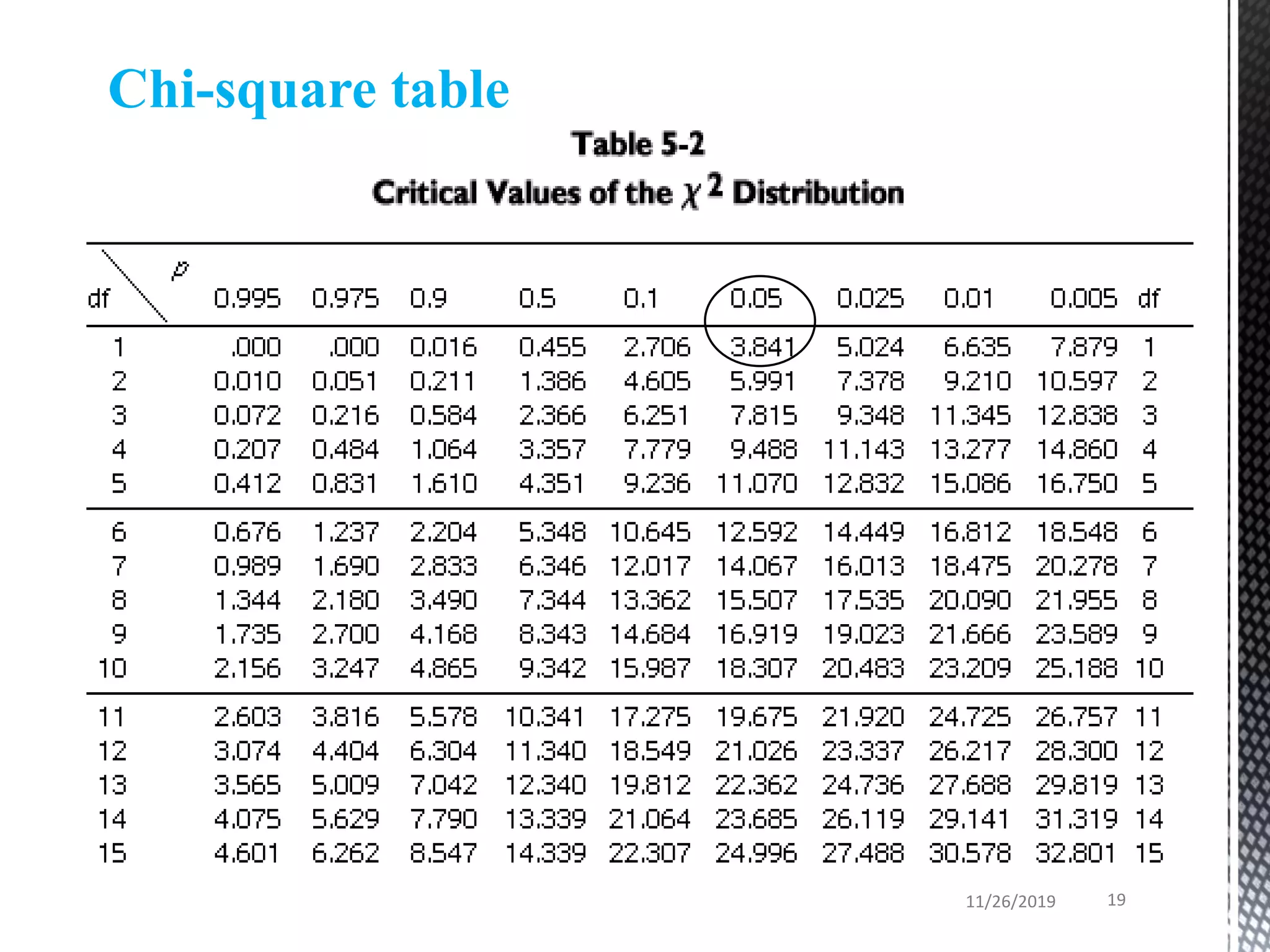
Chi-square distribution and Level of significance (α)
predetermined value
11/26/2019 18](https://image.slidesharecdn.com/categoricaldataanalysis-191127143622/75/Categorical-data-analysis-18-2048.jpg)
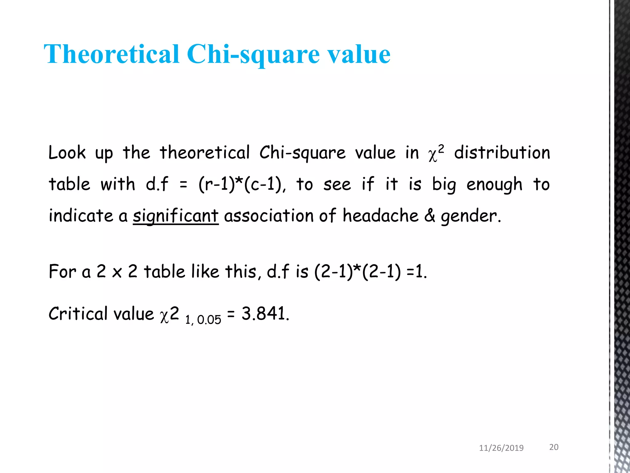
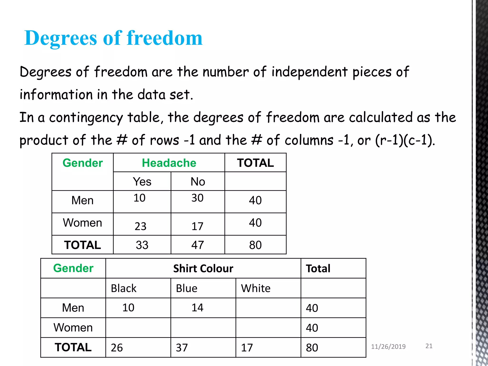
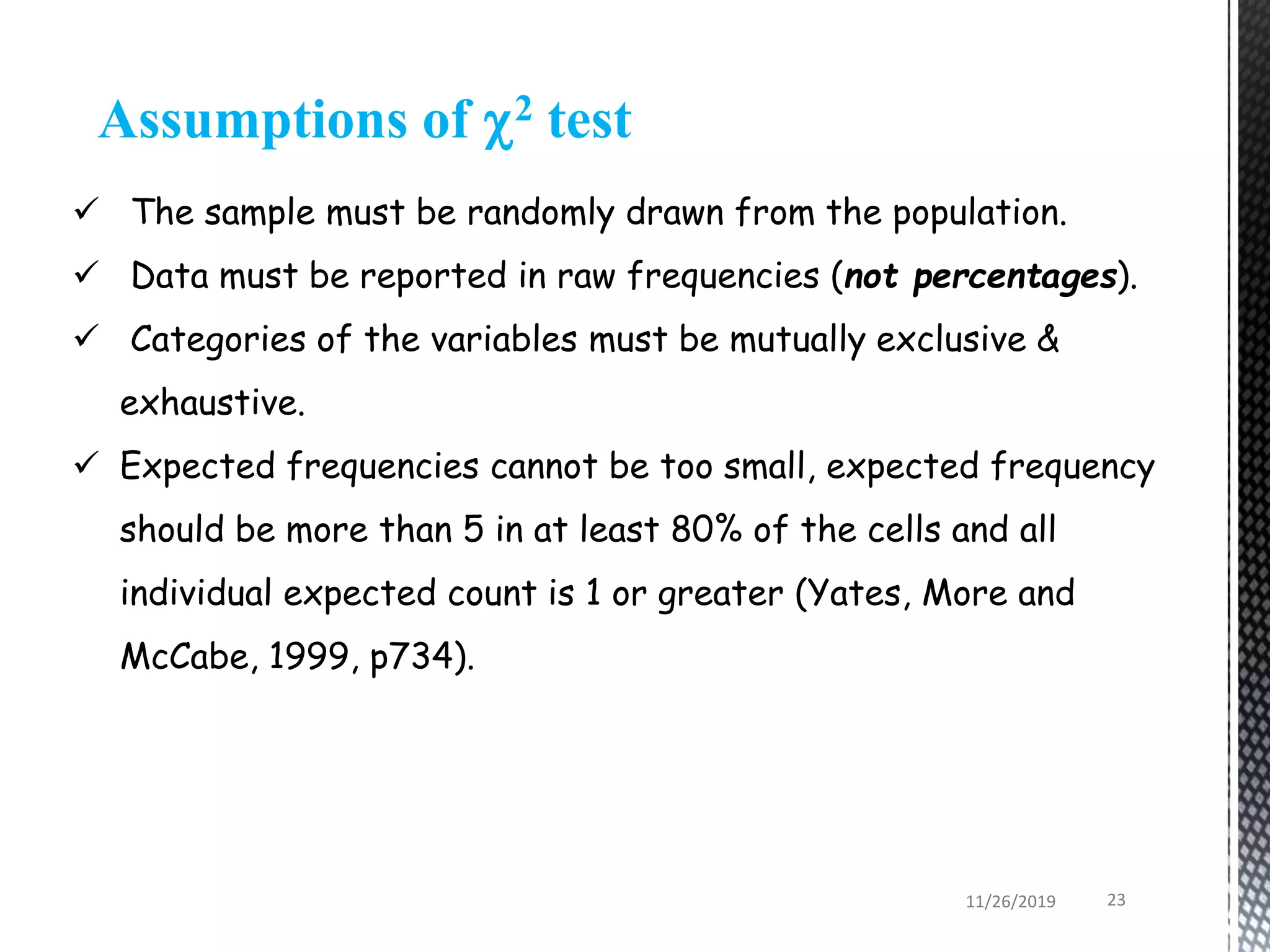
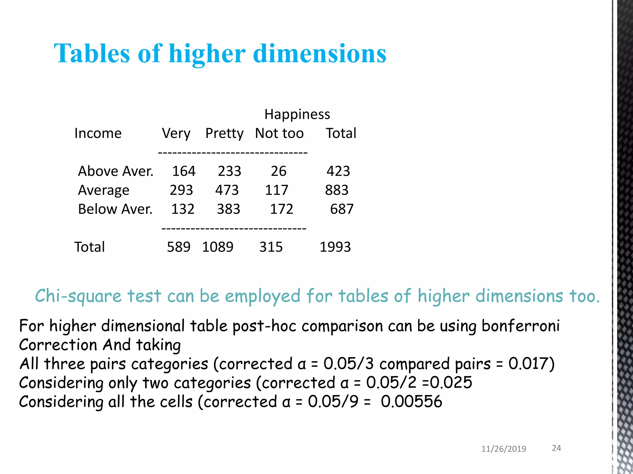
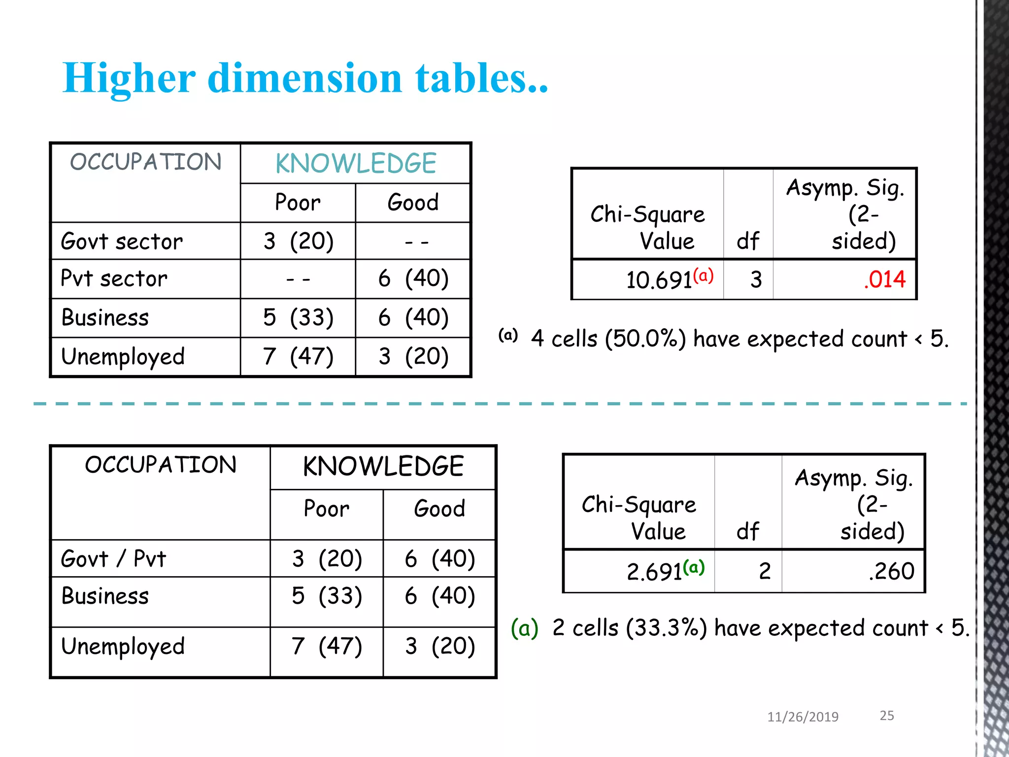
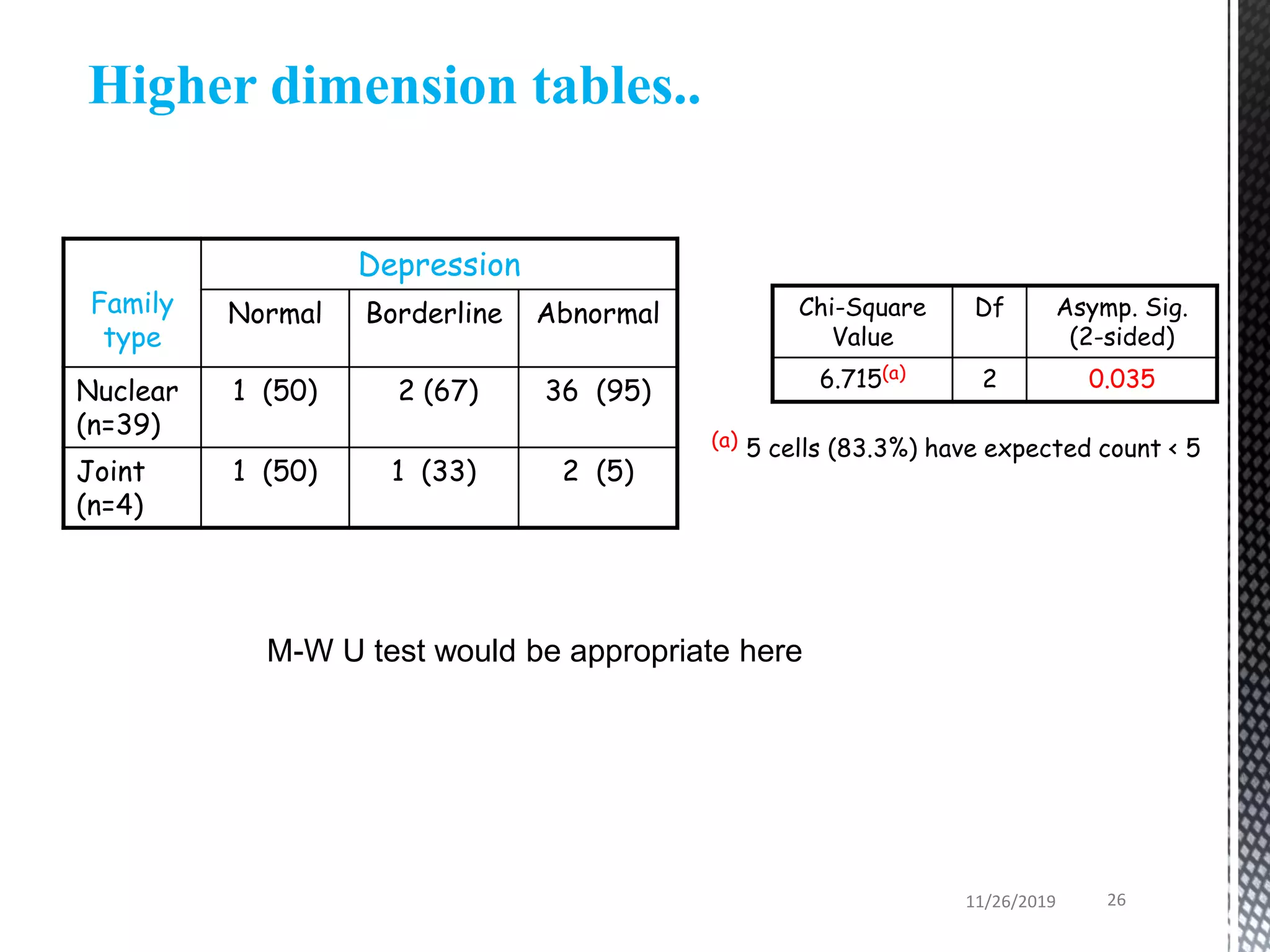
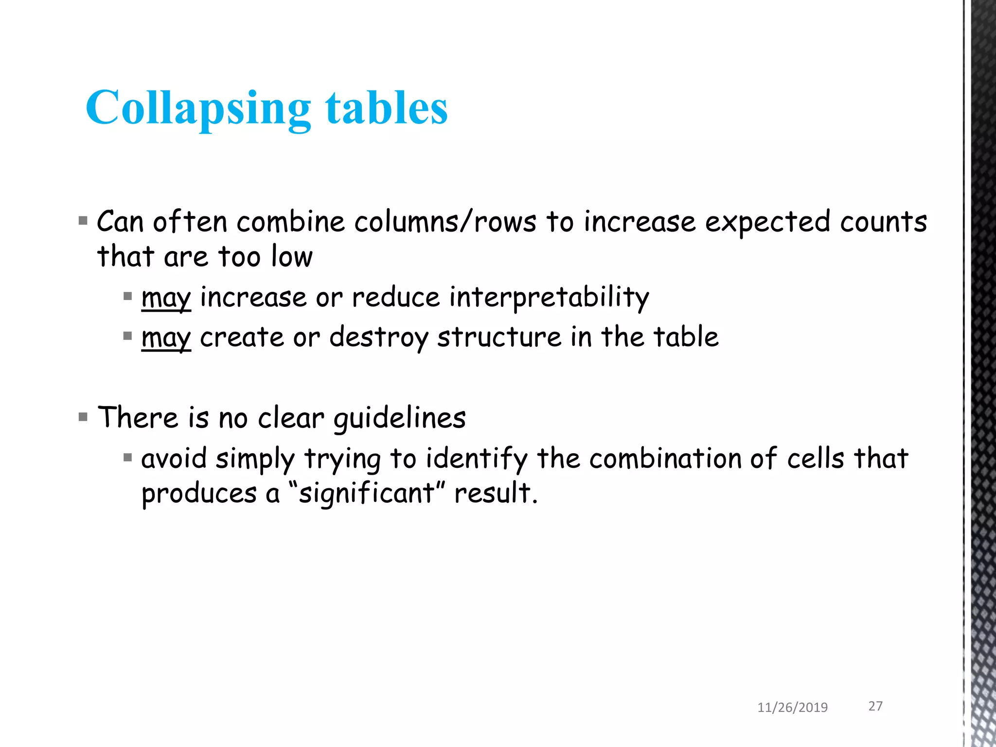
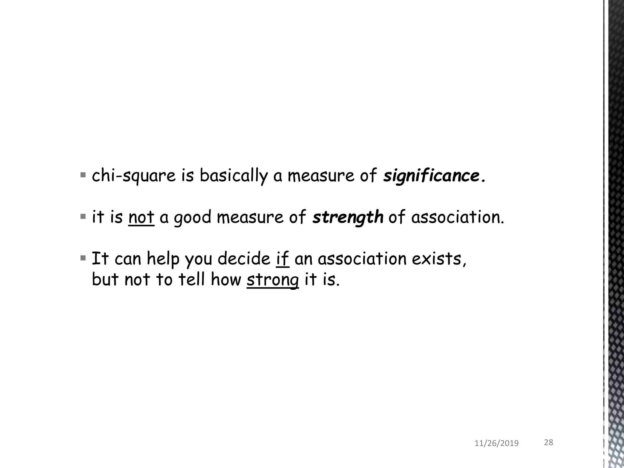
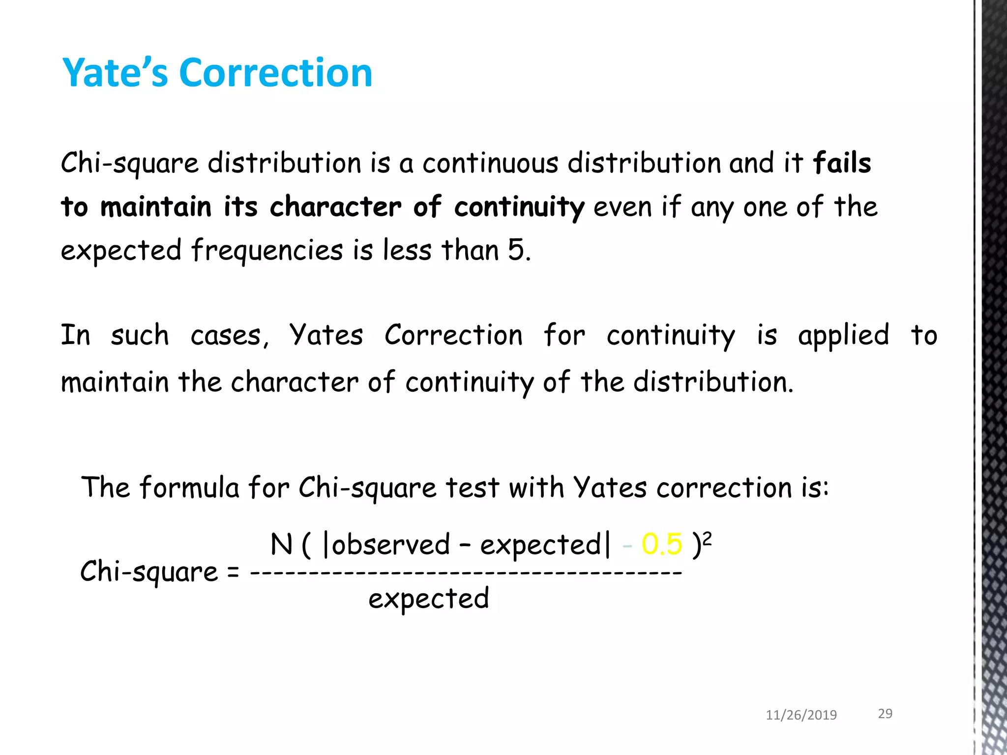
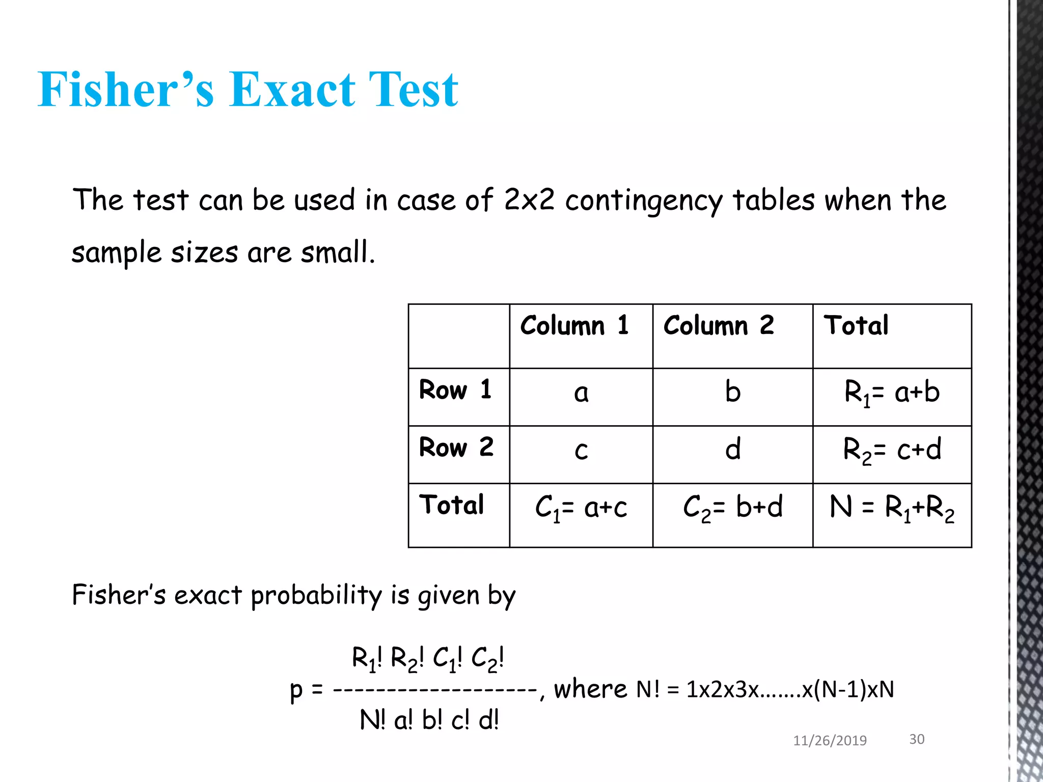

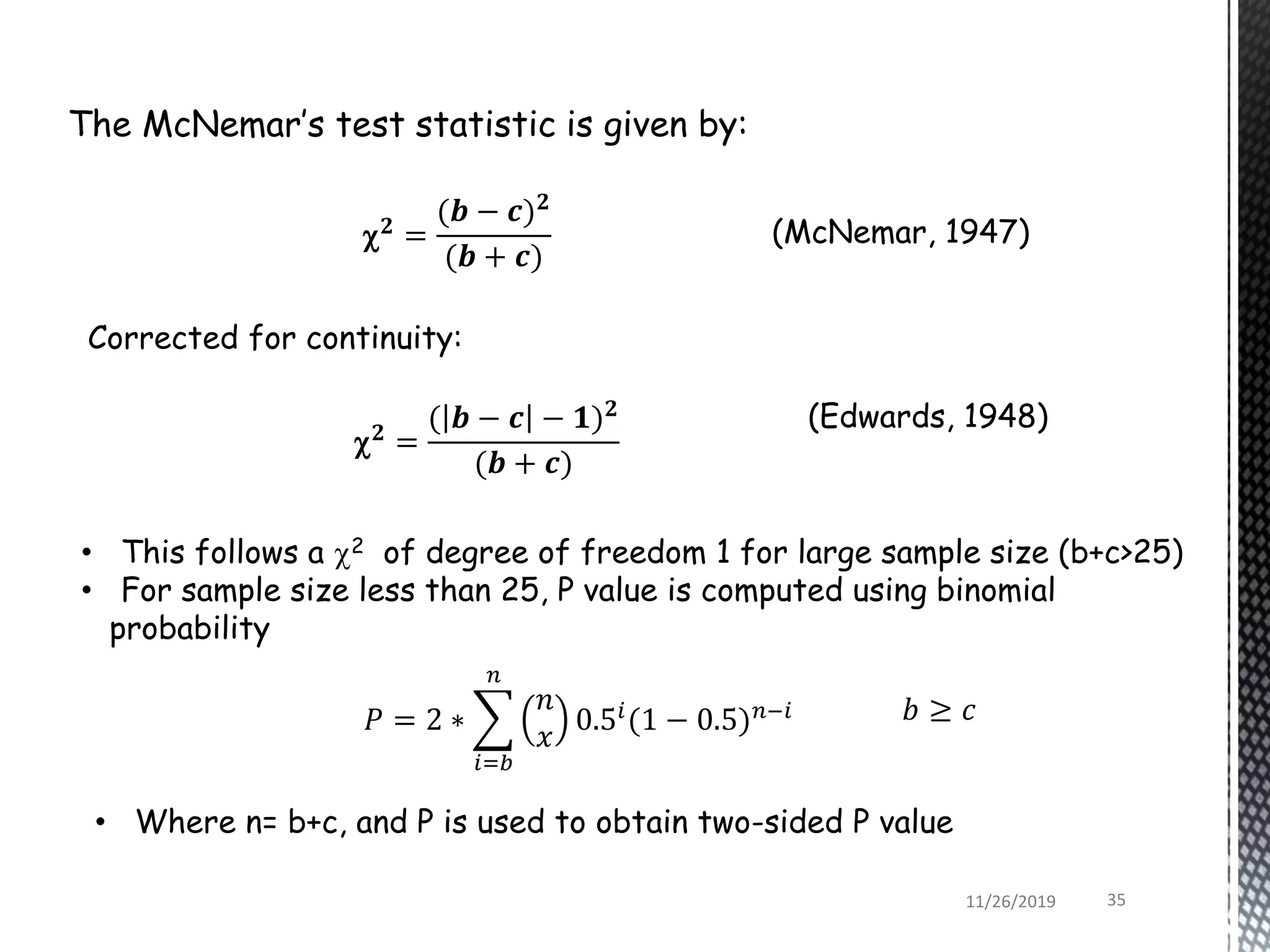

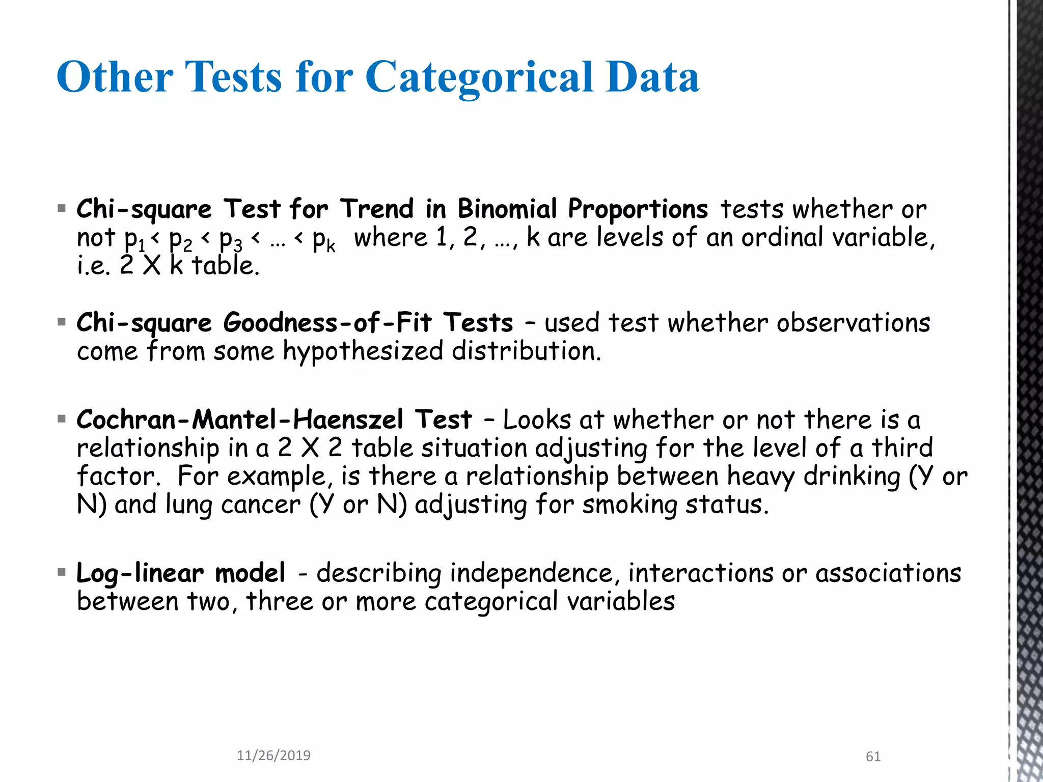


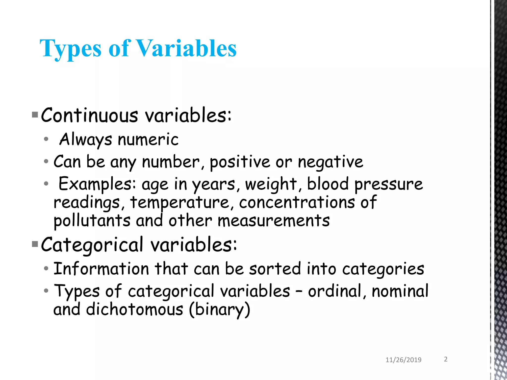
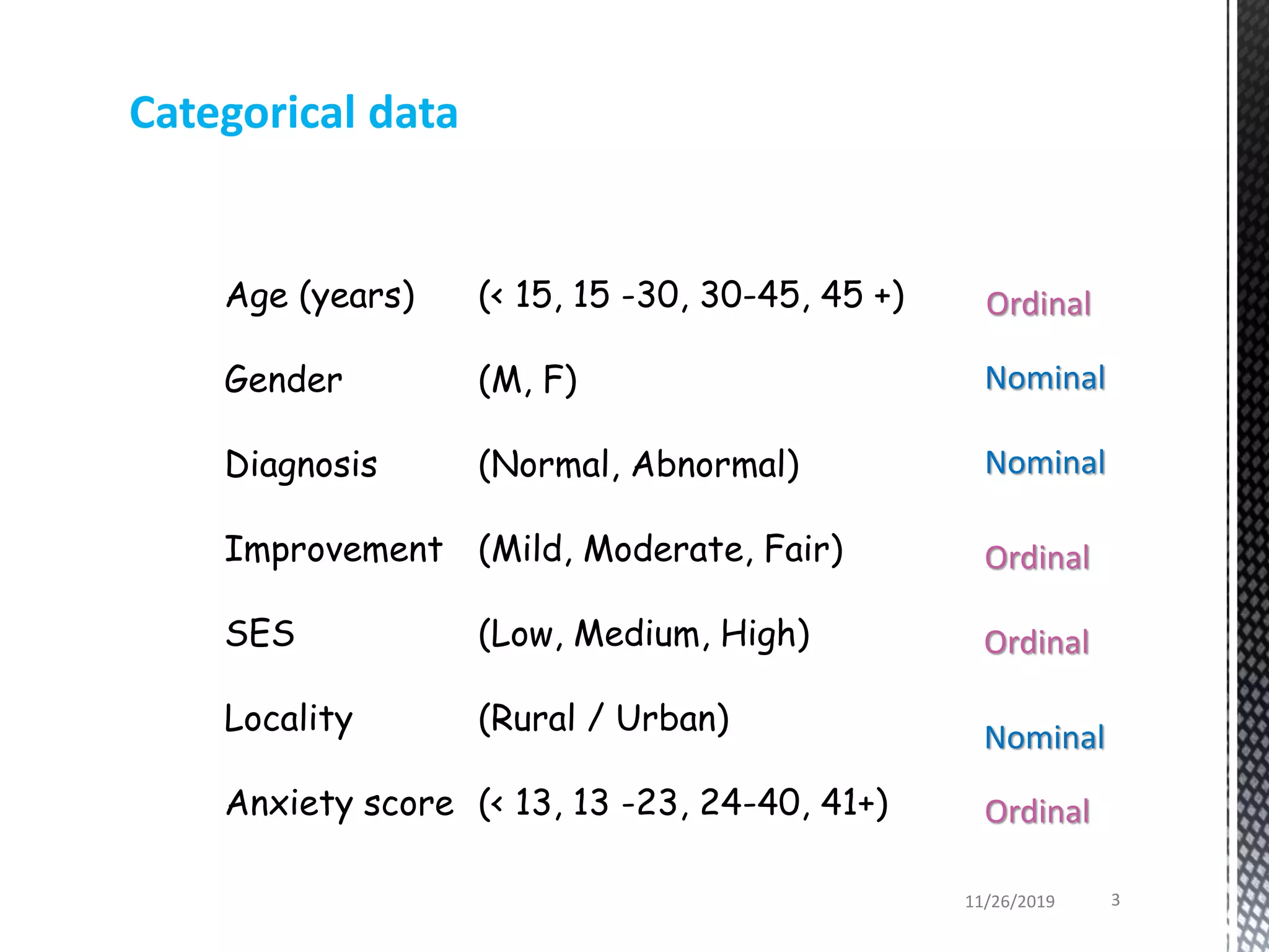
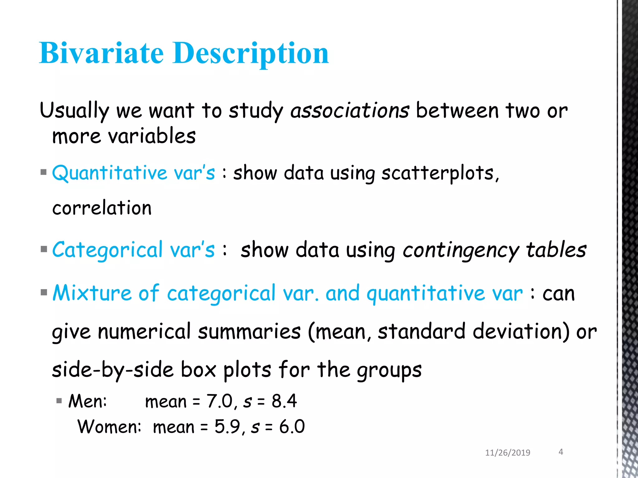
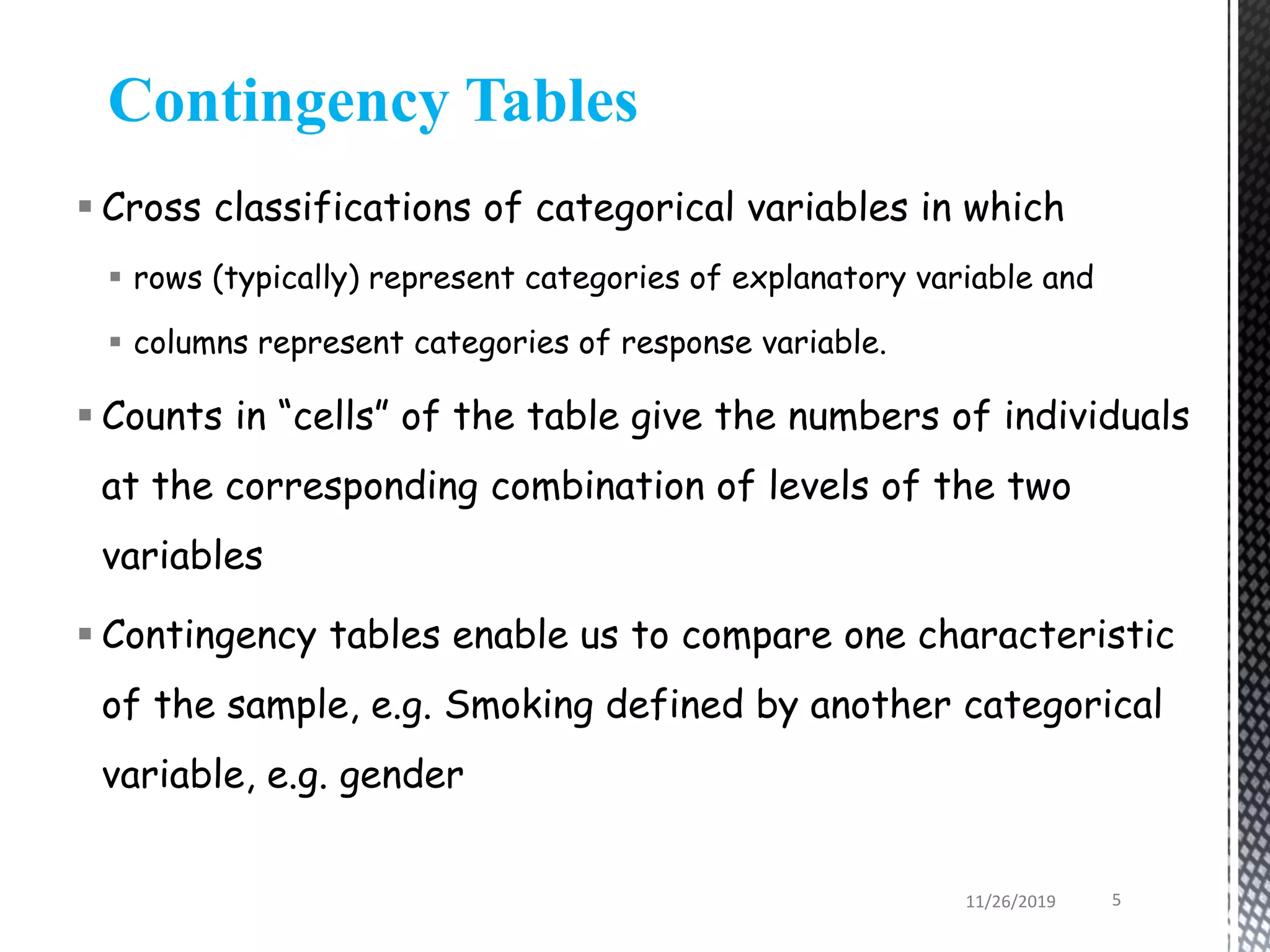
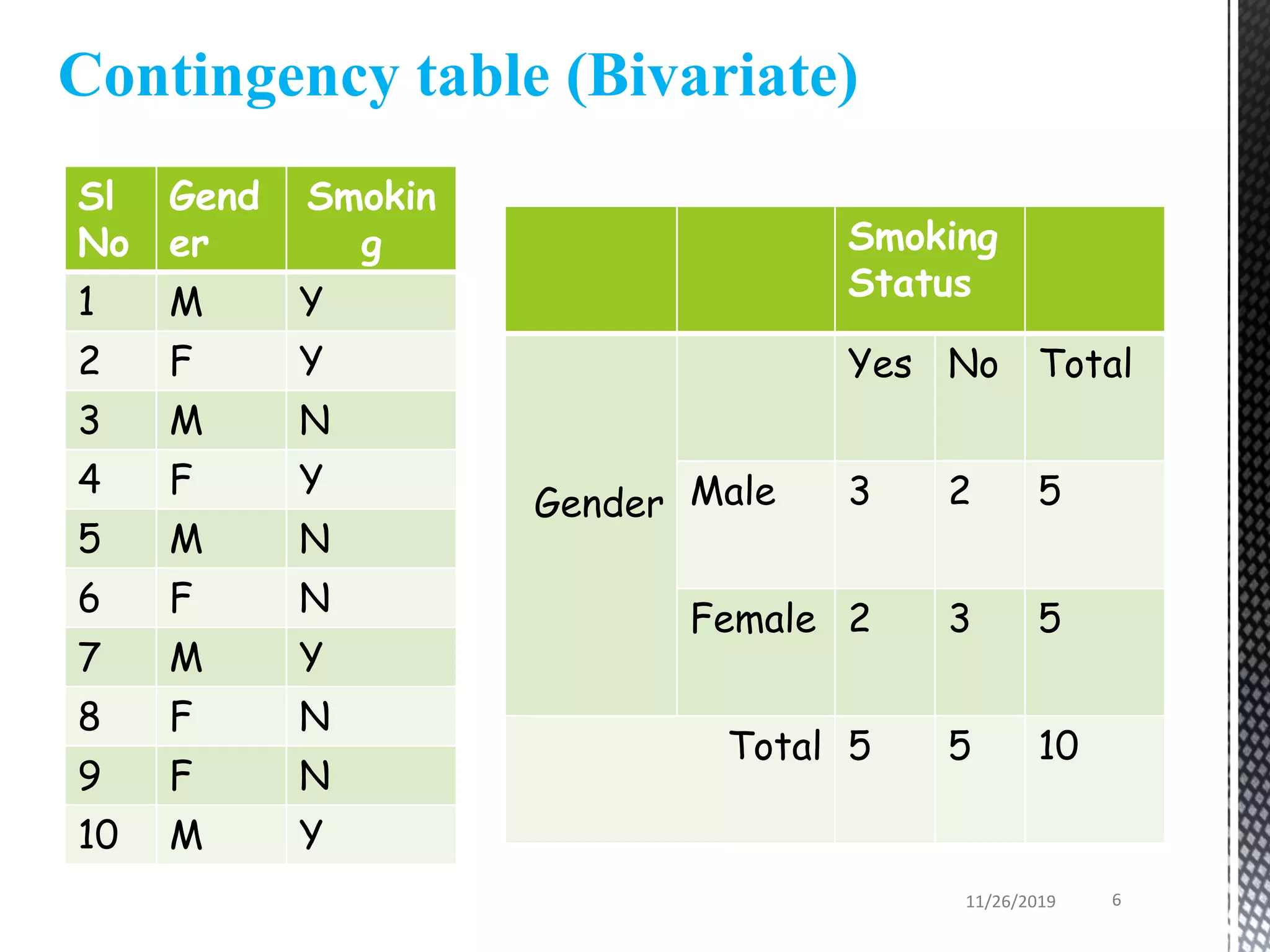
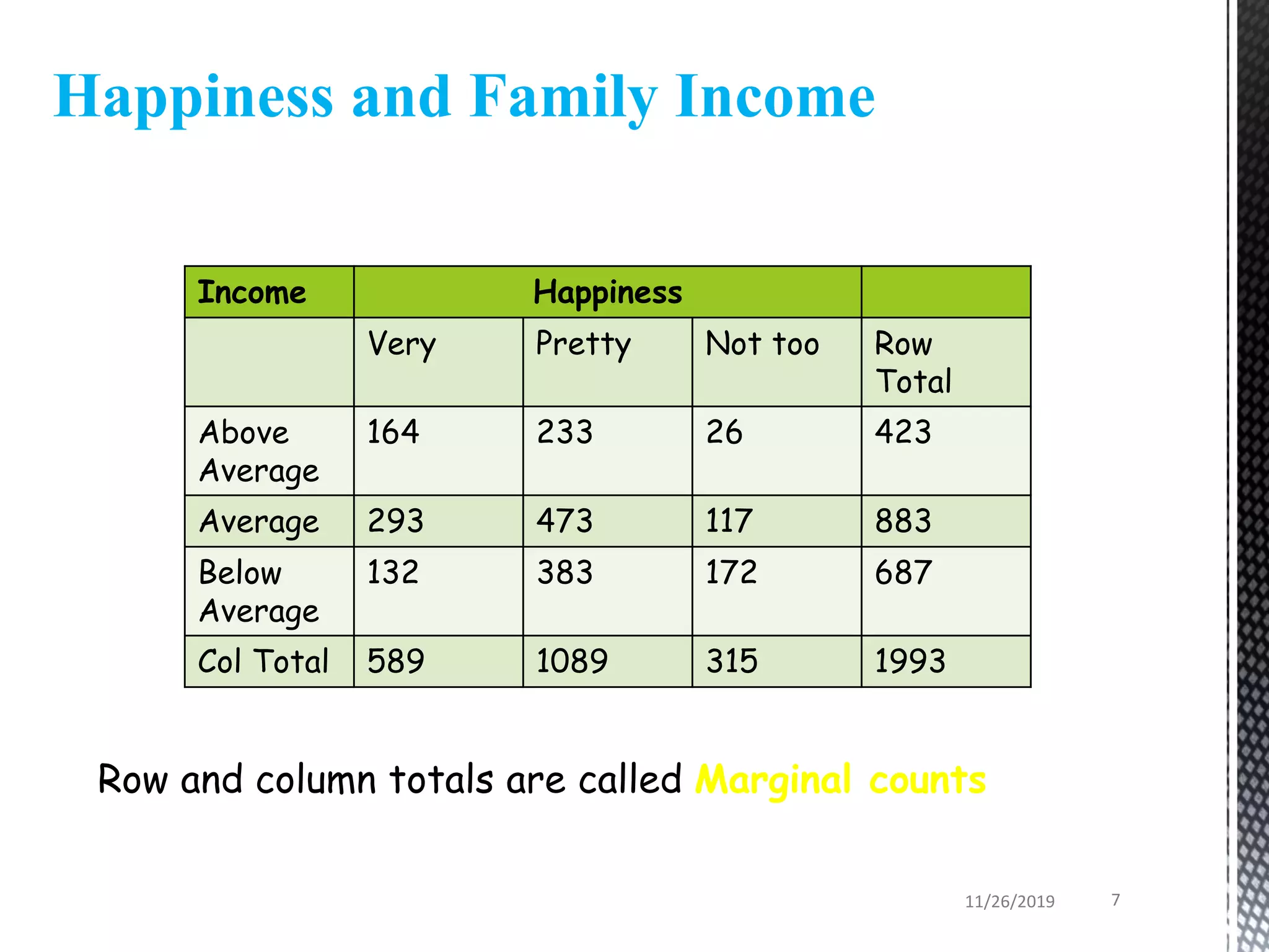
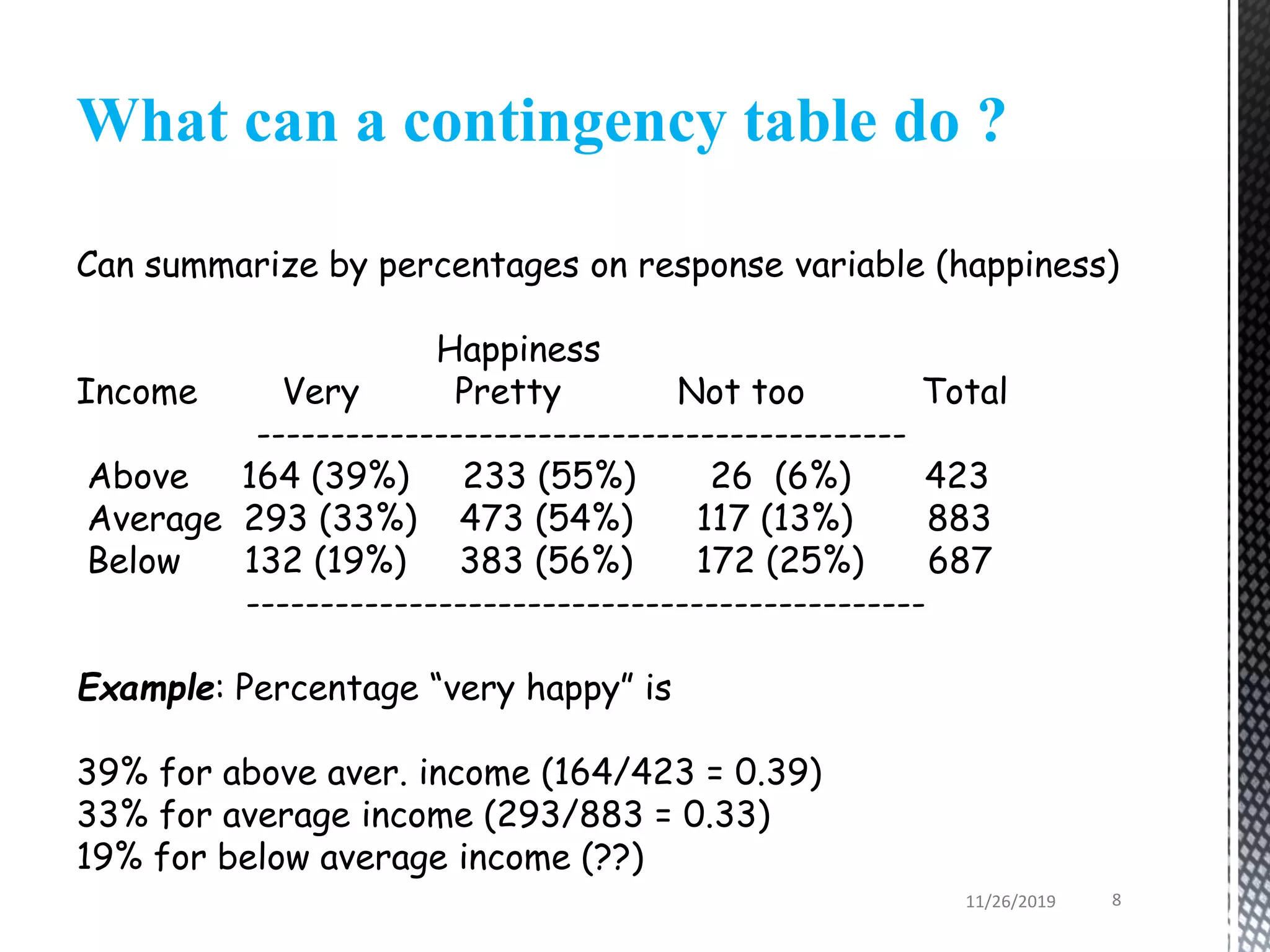
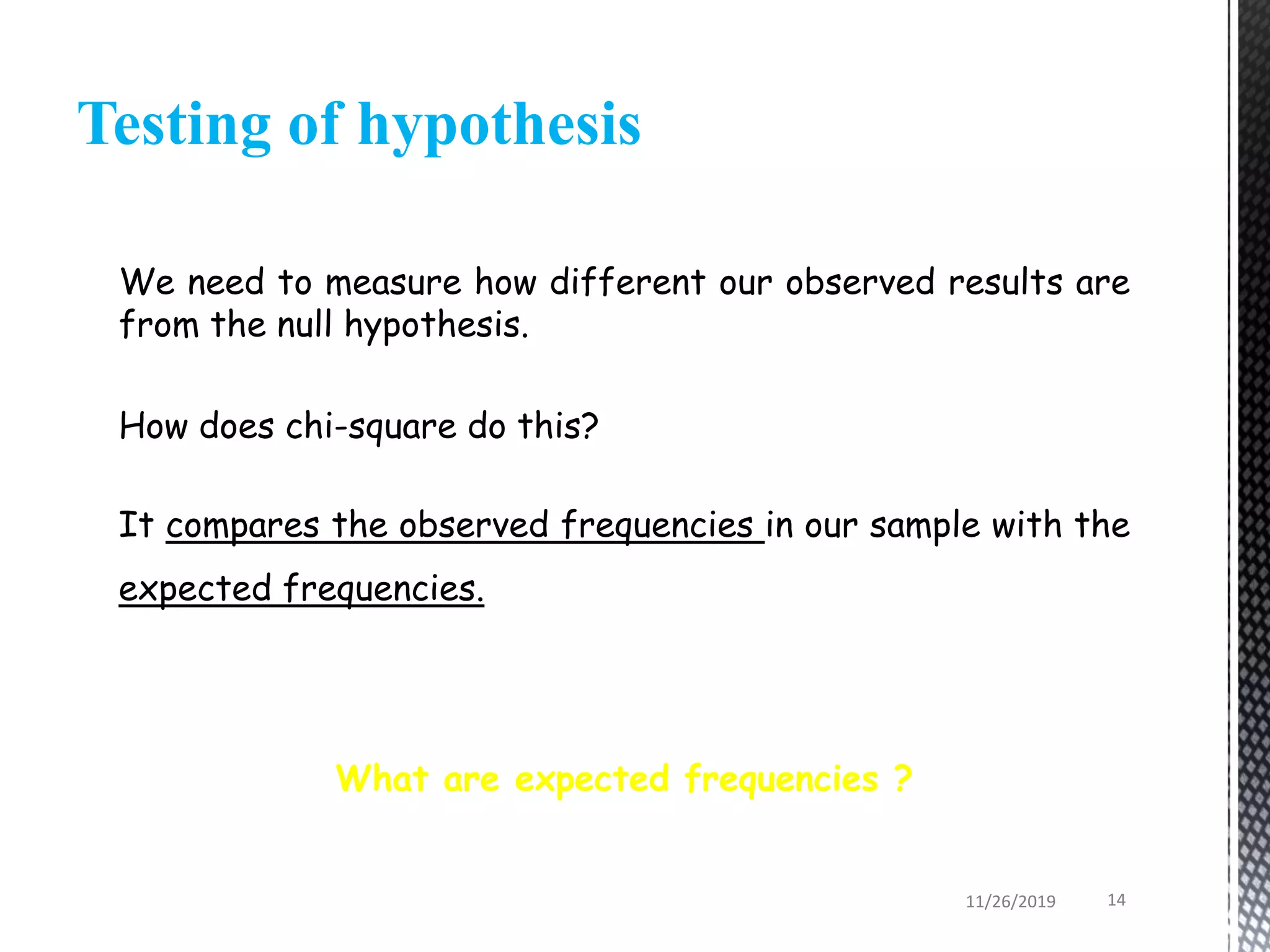
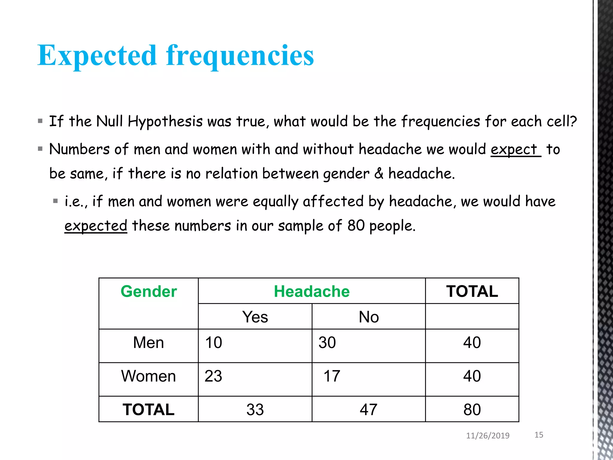
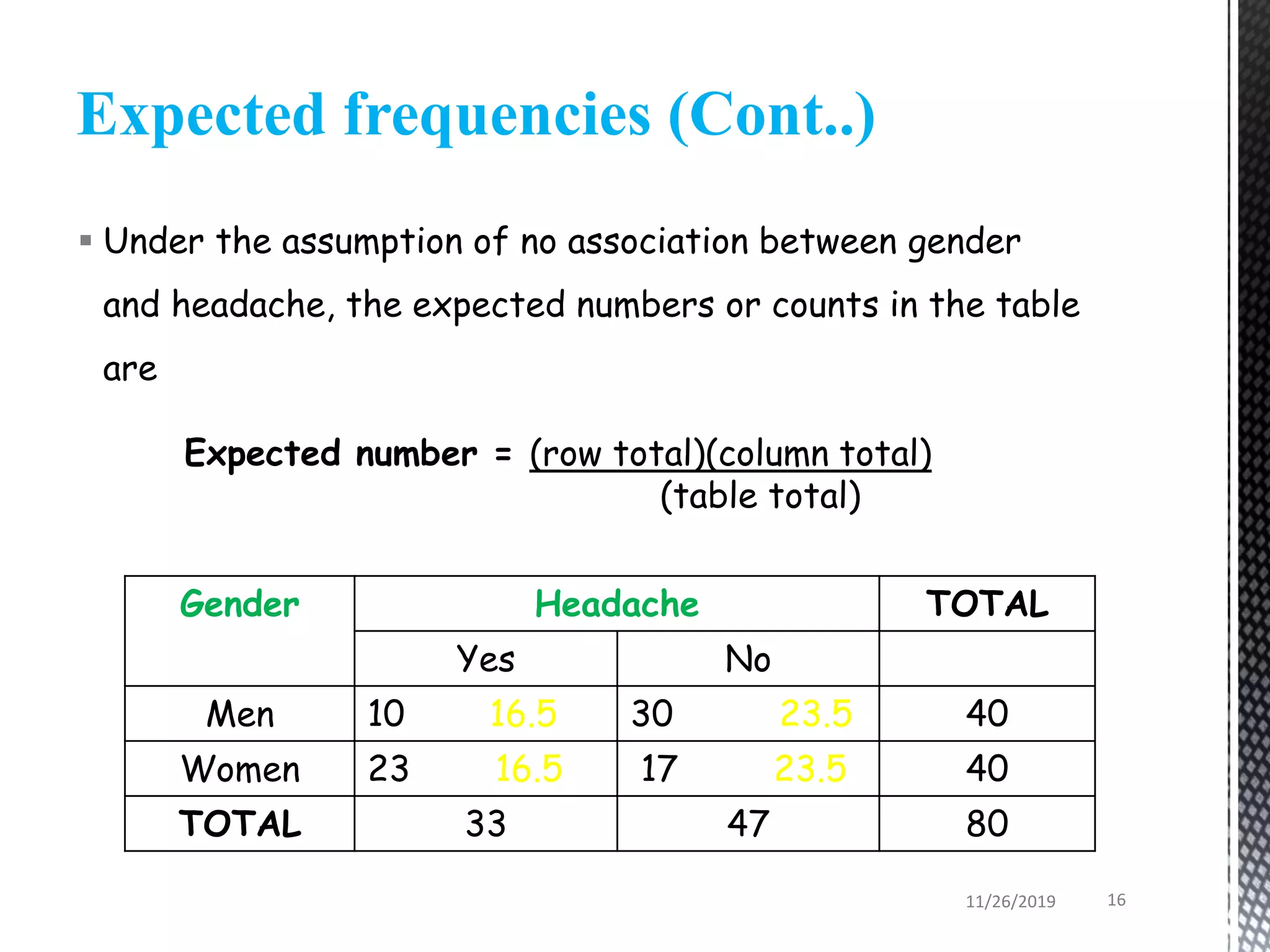
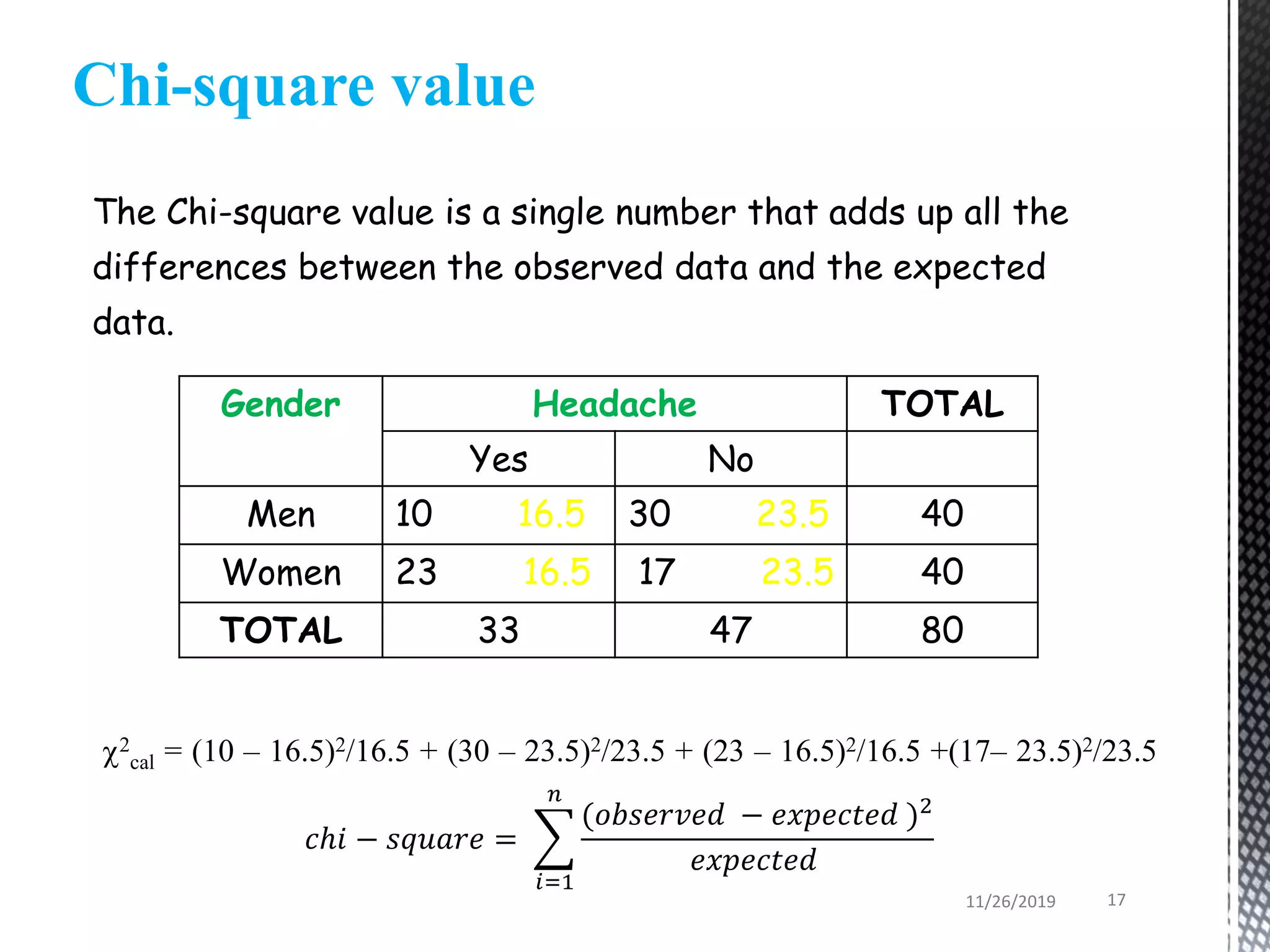
This document discusses various statistical tests used to analyze categorical data, including contingency tables and chi-square tests. It begins by defining continuous and categorical variables. It then discusses how to represent associations between categorical variables using contingency tables. It explains how to calculate expected frequencies and chi-square values to test for relationships between categorical variables. Finally, it discusses other tests that can be used for contingency tables like Fisher's exact test, McNemar's test, and Yates correction.


![Chi square[1]](https://cdn.slidesharecdn.com/ss_thumbnails/chisquare1-150425111505-conversion-gate01-thumbnail.jpg?width=640&height=640&fit=bounds)


