Propensity Score Methods for
Comparative Effectiveness Research with
Multiple Treatment Groups
Kazuki Yoshida
Division of Rheumatology, Immunology and Allergy
Brigham and Women’s Hospital & Harvard Medical School
@kaz_yos kaz-yos kazukiyoshida@mail.harvard.edu
2019-03-18 at
Study Design and Biostatistics Center
Department of Population Health Sciences
University of Utah
1 / 50
Multi-group Comparative Effectiveness
Increasing availability of multiple medications
=⇒ Need for CER involving multiple groups.
Recent observational CER examples in literature:
[Zeng et al., 2019] Analgesics: Tramadol, Naproxen,
Diclofenac, Celecoxib, Etoricoxib, Codeine
[Pawar et al., 2019] Biological Antirheumatics:
Tocilizumab, Tumor necrosis factor inhibitors, Abatacept
[Bergstra et al., 2019] Antirheumatics: Synthetic,
Synthetic + Glucocorticoids, Biological w or w/o
synthetic
[Shah et al., 2018] Anticoagulants: Rivaroxaban,
Dabigatran, Apixaban, Warfarin
6 / 50
Propensity Score Methods and CER
Propensity score (PS) [Rosenbaum and Rubin, 1983]
methods are routinely used in CER comparing two
treatment strategies.
Adjustment [Rosenbaum and Rubin, 1983]
Stratification [Rosenbaum and Rubin, 1984]
Matching [Rosenbaum and Rubin, 1985]
Weighting [Rosenbaum, 1987]
However, when there are more than two treatment
strategies of interest, adaptation is less clear and varies
across fields. [Lopez and Gutman, 2017]
7 / 50
Approaches in Examples
Paper Treatment Approach
[Zeng et al., 2019] Analgesics Pairwise PS, Match
[Pawar et al., 2019] Biologics Pairwise PS, Match
[Bergstra et al., 2019] Antirheumatics Multinom PS, Adjust
[Shah et al., 2018] Anticoagulants Pairwise PS, Adjust
Several options in multi-group CER.
Cohort Construction: Pairwise vs Simultaneous eligibility
PS Estimation: Binary vs Multinomial (logistic) model
PS Methods: Adjustment, Stratification, Matching, or
Weighting
8 / 50
Example of RCT with Multiple Groups
Prospective Randomized Evaluation of Celecoxib
Integrated Safety versus Ibuprofen or Naproxen
(PRECISION) trial [Becker et al., 2009, Nissen et al., 2016]
9 / 50
Question
How can we better design multi-group CER using PS
methods?
10 / 50
Two-Group PS
Weighting
11 / 50
Notations
Yi : Outcome
Ai : Treatment Strategy
Xi : Vector of Covariates
ei : Propensity Score
where
ei = P[Ai = 1|Xi ]
12 / 50
Balancing Weights
[Li et al., 2018] organized existing PS weighting strategies
as a class of weights (covariate) "balancing weights".
The balancing weight for a given individual is defined as:
h(Xi )
Ai ei + (1 − Ai )(1 − ei )
= h(Xi )IPTWi
where h(·) is a prespecified scalar function of Xi , but not Ai .
Intuition:
Denominator (IPTW) balances groups in covariates
Numerator h(·) manipulates target population (estimand)
13 / 50
PS Weighting with Binary Strategy
IPTWi =
1
Ai ei + (1 − Ai )(1 − ei )
=
⎧
⎪⎪⎨
⎪⎪⎩
1
ei
for Ai = 1
1
1 − ei
for Ai = 0
ATTWi =
ei
Ai ei + (1 − Ai )(1 − ei )
=
⎧
⎨
⎩
1 for Ai = 1
ei
1 − ei
for Ai = 0
ATUWi =
1 − ei
Ai ei + (1 − Ai )(1 − ei )
=
⎧
⎨
⎩
1 − ei
ei
for Ai = 1
1 for Ai = 0
MWi =
min {ei , 1 − ei }
Ai ei + (1 − Ai )(1 − ei )
=
ATTWi for ei ≤ 0.5
ATUWi for ei > 0.5
OWi =
ei (1 − ei )
Ai ei + (1 − Ai )(1 − ei )
=
1 − ei for Ai = 1
ei for Ai = 0
[Rosenbaum, 1987, Robins et al., 2000, Sato and Matsuyama, 2003, Li and Greene, 2013,
Li et al., 2018]
14 / 50
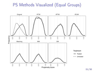
PS Methods Visualized (Equal Groups)
Matching MW OW
Original IPTW ATTW ATUW
0.0
0.5
1.0
0.0
0.5
1.0
0.0
0.5
1.0
0.0
0.5
1.0
0.0
0.5
1.0
0.0
0.5
1.0
0.0
0.5
1.0
Propensity score
Frequency
Treatment
Treated
Untreated
15 / 50
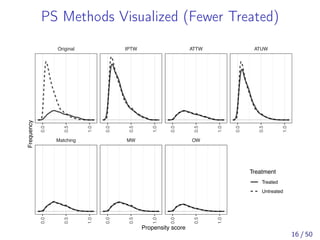
PS Methods Visualized (Fewer Treated)
Matching MW OW
Original IPTW ATTW ATUW
0.0
0.5
1.0
0.0
0.5
1.0
0.0
0.5
1.0
0.0
0.5
1.0
0.0
0.5
1.0
0.0
0.5
1.0
0.0
0.5
1.0
Propensity score
Frequency
Treatment
Treated
Untreated
16 / 50
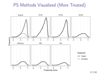
PS Methods Visualized (More Treated)
Matching MW OW
Original IPTW ATTW ATUW
0.0
0.5
1.0
0.0
0.5
1.0
0.0
0.5
1.0
0.0
0.5
1.0
0.0
0.5
1.0
0.0
0.5
1.0
0.0
0.5
1.0
Propensity score
Frequency
Treatment
Treated
Untreated
17 / 50
Asymptotic Equivalence of MW and 1:1 PSM
[Li and Greene, 2013] proved the asymptotic equivalence
of the MW estimand and 1:1 PS matching estimand
under:
Finite PS space (no growth with n)
Positivity (i.e., perfect overlap)
1:1 exact PS matching
18 / 50
Estimands
Using balancing weights [Li et al., 2018] various
population can be targeted for inference of the (marginal)
treatment effect.
IPTW targets average treatment effect (ATE).
We can weights specifically for the average treatment
effect on the treated (ATT) or untreated (ATU)
1:1 PSM and MW target the treatment effect in a
feasible subset of the sample.
[Samuels and Greevy, 2018] named this estimand
"average treatment effect on the evenly matchable units"
(ATM).
OW similarly targets a feasible subset.
19 / 50
Multiple Group
Setting
20 / 50
Generalized PS
Conditional probability of receiving a particular level of
the treatment given the pre-treatment variables:
[Imbens, 2000]
Ai ∈ {0, 1, ..., J}
eji = P[Ai = j|Xi ]
Subject to
J
j=0
eji = 1
Each individual has a PS vector ei = (e0i , e1i , . . . , eJi )T
.
21 / 50
Generalized Balancing Weights
[Li and Li, 2018] extended the balancing weights
framework using the generalized PS.
Using our notation,
h(Xi )
J
j=0
eji I(Ai = j)
= h(Xi )IPTWi
where h(·) is a prespecified scalar function of Xi , but not Ai .
Intuition:
Denominator (IPTW) balances groups in covariates
Numerator h(·) manipulates target population (estimand)
22 / 50
Generalized PS Weighting
IPTWi =
1
J
j=0
eji I(Ai = j)
=
1
eAi i
> 1 for all Ai
AT(k)Wi =
eji
J
j=0
eki I(Ai = j)
=
⎧
⎨
⎩
1 for Ai = k
eki
eAi i
for Ai ̸= k
MWi =
minj {eji }
J
j=0
eji I(Ai = j)
=
⎧
⎨
⎩
1 for Ai = argminj {eji }
minj {eji }
eAi i
< 1 otherwise
OWi =
J
j=0
1
eji
−1
J
j=0
eji I(Ai = j)
=
⎧
⎨
⎩
1
eAi i
1
J
l=0
1
eli
< 1 for all Ai = 1
[Yoshida et al., 2017, Li and Li, 2018]
23 / 50
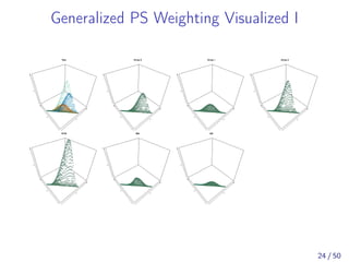
Generalized PS Weighting Visualized I
x
y
z
Raw
xy
z
Group 0
x
y
z
Group 1
x
y
z
Group 2
x
y
z
IPTW
x
y
z
MW
xy
z
OW
24 / 50
Generalized PS Weighting Visualized II
x
y
z
Raw
x
y
z
Group 0
x
y
z
Group 1
x
y
z
Group 2
x
y
z
IPTW
x
y
z
MW
x
y
z
OW
25 / 50
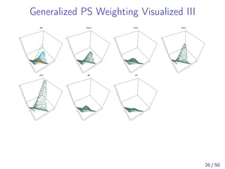
Generalized PS Weighting Visualized III
x
y
z
Raw
x
y
z
Group 0
x
y
z
Group 1
x
y
z
Group 2
x
y
z
IPTW
x
y
z
MW
x
y
z
OW
26 / 50
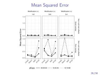
Simulation Study
[Yoshida et al., 2017] examined 3-group MW in
comparison to 3-group IPTW and 1:1:1 simultaneous
three-way matching [Rassen et al., 2013].
OW was not included.
27 / 50
Mean Squared Error
●●●
●●●
●●● ●●●
●
●●
●
●
●
●
●●
●
●
●
●●● ●
●●
●●● ●●●
●
●
●
●
●
●
●
●
●
●
●
●
●●● ●
●●
●●● ●●●
●
●
● ●
●
●
●
●●
●
●
●
Modification (+)
1v0
Modification (+)
2v0
Modification (+)
2v1
Goodoverlap
Non−nullmaineffects
Pooroverlap
Non−nullmaineffects
U
nadj
M
atch
M
W
IPTW
U
nadj
M
atch
M
W
IPTW
U
nadj
M
atch
M
W
IPTW
0.0
0.5
1.0
1.5
0.0
0.5
1.0
1.5
MeanSquaredError
pExpo 33:33:33 10:45:45 10:10:80
28 / 50
Estimands
Modification (+)
1v0
Modification (+)
2v0
Modification (+)
2v1
Goodoverlap
Non−nullmaineffects
Pooroverlap
Non−nullmaineffects
U
nadj
M
atch
M
W
IPTW
U
nadj
M
atch
M
W
IPTW
U
nadj
M
atch
M
W
IPTW
0.40
0.50
0.75
1.00
0.40
0.50
0.75
1.00
TrueRiskRatio
pExpo 33:33:33 10:45:45 10:10:80
Estimand calculation was based on the counterfactual method described in [Austin, 2013] 29 / 50
Simulation: Summary results
Comparing MW to three-way matching and IPTW, we found:
Similar estimands for MW and matching, but not IPTW
Best covariate balance
Similarly small bias compared to matching
Smaller MSE compared to matching in all scenarios
More robust to rare events, unequally sized groups, and
poor covariate overlap
The full results are available in [Yoshida et al., 2017]
30 / 50
Empirical example
Medicare Beneficiary dataset from PA and NJ
(1999-2005) [Solomon et al., 2010]
Unadjusted
nsNSAIDs Coxibs Opioids SMD
n 4874 6172 12601
Charlson score, mean (SD) 1.59 (1.54) 1.72 (1.53) 2.17 (1.78) 0.23
Antithrombotic use, % 14.4 17.6 27.7 0.22
No. prescription drugs, mean (SD) 8.28 (4.69) 8.55 (4.76) 9.76 (5.38) 0.20
No. days in hospital, mean (SD) 1.85 (6.90) 2.19 (6.86) 4.18 (9.46) 0.19
White race, % 84.6 88 92.4 0.16
Fracture, % 6.5 7.2 13.7 0.16
Loop diuretic use, % 21.3 25.8 31.3 0.15
Age, mean (SD) 79.67 (7.03) 80.87 (6.99) 81.15 (7.17) 0.14
No. physician visits, mean (SD) 8.72 (6.32) 8.80 (5.99) 10.08 (7.14) 0.14
Myocardial infarction, % 5.2 5.7 9.6 0.11
Stroke, % 15.2 16.1 21.5 0.11
31 / 50
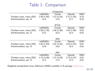
Table 1: Comparison
Unadjusted
nsNSAIDs Coxibs Opioids SMD
Charlson score, mean (SD) 1.59 (1.54) 1.72 (1.53) 2.17 (1.78) 0.23
Antithrombotic use, % 14.4 17.6 27.7 0.22
IPTW
nsNSAIDs Coxibs Opioids SMD
Charlson score, mean (SD) 1.98 (1.70) 1.94 (1.68) 1.94 (1.69) 0.02
Antithrombotic use, % 23.3 22.5 22.4 0.01
MW
nsNSAIDs Coxibs Opioids SMD
Charlson score, mean (SD) 1.62 (1.53) 1.61 (1.52) 1.63 (1.53) 0.01
Antithrombotic use, % 14.9 14.8 15.2 0.01
OW
nsNSAIDs Coxibs Opioids SMD
Charlson score, mean (SD) 1.73 (1.58) 1.71 (1.56) 1.73 (1.57) 0.01
Antithrombotic use, % 17.5 17.2 17.5 0.01
Weighted standardized mean difference (SMD) available in R package tableone.
32 / 50
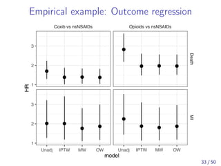
Empirical example: Outcome regression
●
● ● ●
● ●
●
●
●
● ● ●
●
● ● ●
Coxib vs nsNSAIDs Opioids vs nsNSAIDs
DeathMI
Unadj IPTW MW OW Unadj IPTW MW OW
1
2
3
1
2
3
model
HR
33 / 50
Conclusion
MW has been suggested as a more efficient alternative to
1:1 pairwise matching. [Li and Greene, 2013]
In a simulation study with three treatment groups, MW
demonstrated similar bias, but smaller MSE compared to
1:1:1 three-way matching. [Rassen et al., 2013]
Efficiency gain compared to 1:1:1 three-way matching was
more noticeable in scenarios in which the outcome events
were rare, treatment groups were unequally sized, or
covariate overlap was poor.
Compared to IPTW, MW was more stable in the poor
covariate overlap setting.
Confirming the type of patients that MW is making
inference for is important in practice.
34 / 50
PS Trimming
35 / 50
PS Trimming
Propensity score trimming has been suggested by several
authors.
To increase efficiency [Crump et al., 2009]
To reduce unmeasured confounding
[Stürmer et al., 2010]
To guide study design [Walker et al., 2013]
[Yoshida et al., 2019] examined multi-group extension of
all three.
Here we focus on the extension of [Stürmer et al., 2010].
36 / 50
Motivation for Stürmer’s PS Trimming
[Stürmer et al., 2010] was concerned with very
heterogeneous treatment effects in the tails of PS
distribution.
[Kurth et al., 2006] tissue plasminogen activator (t-PA)
use vs no t-PA use in stroke patients. Outcome
in-hospital death. Very high mortality in t-PA users with
lowest probabilities for t-PA.
[Lunt et al., 2009] tumor necrosis factor inhibitor (TNFi)
initiation vs non-TNFi treatment in rheumatoid arthritis
patients. Outcome death. Higher mortality among
non-TNFi users with highest probabilities for TNFi
initiation.
[Stürmer et al., 2010] hypothesized that there may be
higher prevalence of unmeasured confounders that
preferentially introduce more confounding in the tails.
37 / 50
Definition of Stürmer’s PS Trimming
[Stürmer et al., 2010] proposed the asymmetric PS
trimming to remedy this.
Their simulation study confirmed its benefit in bias
reduction if indeed the tails of PS contained higher
prevalence of unmeasured confounders.
38 / 50
Question
[Stürmer et al., 2010] demonstrated benefits of PS
trimming in reducing unmeasured confounding in the
presence of unmeasured confounders that were more
prevalent in the tails of the PS distribution.
How can we conceptualize this issue in the general
setting?
How can we extend their method?
39 / 50
Original Two-Group Definition
Method Existing Binary Definition
Stürmer Is = i ∈ I : ei ∈ F−1
ei |Ai
(0.05|1), F−1
ei |Ai
(0.95|0)
Define the lower threshold using the treated PS
distribution.
Define the upper threshold
Notation Explanation
i ∈ {1, ..., n} index for an individual
I = {1, ..., n} index set for entire sample
Ai ∈ {0, 1} treatment variable
ei = P[Ai = 1|Xi ] propensity score
p = P[Ai = 1] treatment prevalence
F−1
ei |Ai
(x|a) treatment-specific quantile of ei
40 / 50
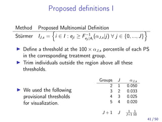
Proposed definitions I
Method Proposed Multinomial Definition
Stürmer IJ,s = i ∈ I : eji ≥ F−1
eji |Ai
(αJ,s|j) ∀ j ∈ {0, ..., J}
Define a threshold at the 100 × αJ,s percentile of each PS
in the corresponding treatment group.
Trim individuals outside the region above all these
thresholds.
We used the following
provisional thresholds
for visualization.
Groups J αJ,s
2 1 0.050
3 2 0.033
4 3 0.025
5 4 0.020
J + 1 J 1
J+1
1
10
41 / 50
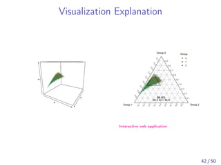
Visualization Explanation
x
y
z
84.6%
(86.2; 82.1; 88.3)
0.1
0.2
0.3
0.4
0.5
0.6
0.7
0.8
0.9
0.1
0.2
0.3
0.4
0.5
0.6
0.7
0.8
0.9
0.1
0.2
0.3
0.4
0.5
0.6
0.7
0.8
0.9
Group 0
Group 1 Group 2
Group
●
●
●
0
1
2
Interactive web application
42 / 50
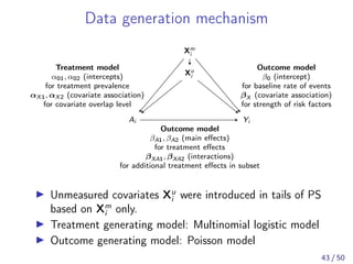
Data generation mechanism
Xm
i
Xu
i
Ai Yi
Outcome model
βA1, βA2 (main effects)
for treatment effects
βXA1, βXA2 (interactions)
for additional treatment effects in subset
Treatment model
α01, α02 (intercepts)
for treatment prevalence
αX1, αX2 (covariate association)
for covariate overlap level
Outcome model
β0 (intercept)
for baseline rate of events
βX (covariate association)
for strength of risk factors
Unmeasured covariates Xu
i were introduced in tails of PS
based on Xm
i only.
Treatment generating model: Multinomial logistic model
Outcome generating model: Poisson model
43 / 50
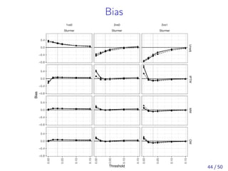
Bias
●
●
●
● ●
●
● ● ● ● ●
●
● ● ● ● ●●
● ● ● ● ●
●
●
●
●
● ●
●
●
● ● ● ●
●
● ● ● ● ●
●
● ● ● ● ●
●
●
●
●
●
●
●
●
● ●
● ●
●
● ● ● ● ●
●
● ● ● ● ●
●
1vs0
Sturmer
2vs0
Sturmer
2vs1
Sturmer
UnadjIPTWMWOW
0.00
0.05
0.10
0.15
0.00
0.05
0.10
0.15
0.00
0.05
0.10
0.15
−0.8
−0.4
0.0
0.4
−0.8
−0.4
0.0
0.4
−0.8
−0.4
0.0
0.4
−0.8
−0.4
0.0
0.4
Threshold
Bias
44 / 50
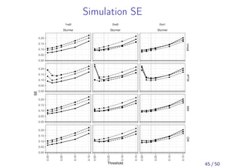
Simulation SE
● ●
●
●
●
●
● ●
●
●
●
●
● ●
●
●
●
●
●
●
●
●
●
●
● ●
●
●
●
●
●
●
●
●
●
●
● ●
●
●
●
●
● ●
●
●
●
●
●
● ●
●
●
●
●
● ●
●
●
●
● ●
●
●
●
●
● ●
●
●
●
●
1vs0
Sturmer
2vs0
Sturmer
2vs1
Sturmer
UnadjIPTWMWOW
0.00
0.05
0.10
0.15
0.00
0.05
0.10
0.15
0.00
0.05
0.10
0.15
0.00
0.05
0.10
0.15
0.20
0.00
0.05
0.10
0.15
0.20
0.00
0.05
0.10
0.15
0.20
0.00
0.05
0.10
0.15
0.20
Threshold
SE
45 / 50
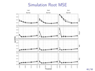
Simulation Root MSE
●
●
●
●
●
●
● ● ● ●
●
●
● ● ● ●
●
●
● ● ● ●
●
●
●
●
●
●
●
●
● ● ●
●
●
●
● ● ●
●
●
●
● ● ●
●
●●
●
●
●
●
●
●
●
● ● ●
●
●
● ● ● ●
●
●
●
● ● ●
●●
1vs0
Sturmer
2vs0
Sturmer
2vs1
Sturmer
UnadjIPTWMWOW
0.00
0.05
0.10
0.15
0.00
0.05
0.10
0.15
0.00
0.05
0.10
0.15
0.0
0.2
0.4
0.6
0.8
0.0
0.2
0.4
0.6
0.8
0.0
0.2
0.4
0.6
0.8
0.0
0.2
0.4
0.6
0.8
Threshold
sqrt(MSE)
46 / 50
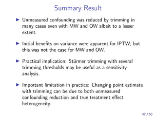
Summary Result
Unmeasured confounding was reduced by trimming in
many cases even with MW and OW albeit to a lesser
extent.
Initial benefits on variance were apparent for IPTW, but
this was not the case for MW and OW.
Practical implication: Stürmer trimming with several
trimming thresholds may be useful as a sensitivity
analysis.
Important limitation in practice: Changing point estimate
with trimming can be due to both unmeasured
confounding reduction and true treatment effect
heterogeneity.
47 / 50
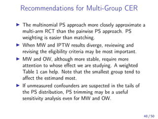
Recommendations for Multi-Group CER
The multinomial PS approach more closely approximate a
multi-arm RCT than the pairwise PS approach. PS
weighting is easier than matching.
When MW and IPTW results diverge, reviewing and
revising the eligibility criteria may be most important.
MW and OW, although more stable, require more
attention to whose effect we are studying. A weighted
Table 1 can help. Note that the smallest group tend to
affect the estimand most.
If unmeasured confounders are suspected in the tails of
the PS distribution, PS trimming may be a useful
sensitivity analysis even for MW and OW.
48 / 50
Further Information on MW
Slides: https://www.slideshare.net/kaz_yos
Code: https://github.com/kaz-yos/mw
Weighted tables:
https://github.com/kaz-yos/tableone
Published Paper: Epidemiology 2017;28:387
1 / 7
Further Information on Trimming
Slides: https://www.slideshare.net/kaz_yos
Code: https://github.com/kaz-yos/
multinomial-ps-trimming
Published Paper: Am J Epidemiol. 2019;188:609
2 / 7
Bibliography I
[Austin, 2013] Austin, P. C. (2013).
The performance of different propensity score methods for estimating marginal hazard ratios.
Stat Med, 32(16):2837–2849.
[Becker et al., 2009] Becker, M. C., Wang, T. H., Wisniewski, L., Wolski, K., Libby, P., Lüscher, T. F.,
Borer, J. S., Mascette, A. M., Husni, M. E., Solomon, D. H., Graham, D. Y., Yeomans, N. D.,
Krum, H., Ruschitzka, F., Lincoff, A. M., Nissen, S. E., and PRECISION Investigators (2009).
Rationale, design, and governance of Prospective Randomized Evaluation of Celecoxib Integrated
Safety versus Ibuprofen Or Naproxen (PRECISION), a cardiovascular end point trial of nonsteroidal
antiinflammatory agents in patients with arthritis.
Am. Heart J., 157(4):606–612.
[Bergstra et al., 2019] Bergstra, S. A., Winchow, L.-L., Murphy, E., Chopra, A., Salomon-Escoto, K.,
Fonseca, J. a. E., Allaart, C. F., and Landewé, R. B. M. (2019).
How to treat patients with rheumatoid arthritis when methotrexate has failed? The use of a multiple
propensity score to adjust for confounding by indication in observational studies.
Ann. Rheum. Dis., 78(1):25–30.
[Crump et al., 2009] Crump, R. K., Hotz, V. J., Imbens, G. W., and Mitnik, O. A. (2009).
Dealing with limited overlap in estimation of average treatment effects.
Biometrika, 96(1):187–199.
[Imbens, 2000] Imbens, G. W. (2000).
The role of the propensity score in estimating dose-response functions.
Biometrika, 87(3):706–710.
3 / 7
Bibliography II
[Kurth et al., 2006] Kurth, T., Walker, A. M., Glynn, R. J., Chan, K. A., Gaziano, J. M., Berger, K.,
and Robins, J. M. (2006).
Results of multivariable logistic regression, propensity matching, propensity adjustment, and
propensity-based weighting under conditions of nonuniform effect.
Am. J. Epidemiol., 163(3):262–270.
[Li and Li, 2018] Li, F. and Li, F. (2018).
Propensity Score Weighting for Causal Inference with Multi-valued Treatments.
arXiv:1808.05339 [stat].
[Li et al., 2018] Li, F., Morgan, K. L., and Zaslavsky, A. M. (2018).
Balancing Covariates via Propensity Score Weighting.
Journal of the American Statistical Association, 113(521):390–400.
[Li and Greene, 2013] Li, L. and Greene, T. (2013).
A weighting analogue to pair matching in propensity score analysis.
Int J Biostat, 9(2):215–234.
[Lopez and Gutman, 2017] Lopez, M. J. and Gutman, R. (2017).
Estimation of Causal Effects with Multiple Treatments: A Review and New Ideas.
Statist. Sci., 32(3):432–454.
[Lunt et al., 2009] Lunt, M., Solomon, D., Rothman, K., Glynn, R., Hyrich, K., Symmons, D. P. M.,
Stürmer, T., British Society for Rheumatology Biologics Register, and British Society for
Rheumatology Biologics Register Control Centre Consortium (2009).
Different methods of balancing covariates leading to different effect estimates in the presence of
effect modification.
Am. J. Epidemiol., 169(7):909–917.
4 / 7
Bibliography III
[Nissen et al., 2016] Nissen, S. E., Yeomans, N. D., Solomon, D. H., Lüscher, T. F., Libby, P., Husni,
M. E., Graham, D. Y., Borer, J. S., Wisniewski, L. M., Wolski, K. E., Wang, Q., Menon, V.,
Ruschitzka, F., Gaffney, M., Beckerman, B., Berger, M. F., Bao, W., Lincoff, A. M., and
PRECISION Trial Investigators (2016).
Cardiovascular Safety of Celecoxib, Naproxen, or Ibuprofen for Arthritis.
N. Engl. J. Med., 375(26):2519–2529.
[Pawar et al., 2019] Pawar, A., Desai, R. J., Solomon, D. H., Santiago Ortiz, A. J., Gale, S., Bao, M.,
Sarsour, K., Schneeweiss, S., and Kim, S. C. (2019).
Risk of serious infections in tocilizumab versus other biologic drugs in patients with rheumatoid
arthritis: A multidatabase cohort study.
Ann. Rheum. Dis.
[Rassen et al., 2013] Rassen, J. A., Shelat, A. A., Franklin, J. M., Glynn, R. J., Solomon, D. H., and
Schneeweiss, S. (2013).
Matching by propensity score in cohort studies with three treatment groups.
Epidemiology, 24(3):401–409.
[Robins et al., 2000] Robins, J. M., Hernán, M. A., and Brumback, B. (2000).
Marginal structural models and causal inference in epidemiology.
Epidemiology, 11(5):550–560.
[Rosenbaum, 1987] Rosenbaum, P. R. (1987).
Model-Based Direct Adjustment.
Journal of the American Statistical Association, 82(398):387–394.
[Rosenbaum and Rubin, 1983] Rosenbaum, P. R. and Rubin, D. B. (1983).
The central role of the propensity score in observational studies for causal effects.
Biometrika, 70(1):41–55.
5 / 7
Bibliography IV
[Rosenbaum and Rubin, 1984] Rosenbaum, P. R. and Rubin, D. B. (1984).
Reducing Bias in Observational Studies Using Subclassification on the Propensity Score.
J Am Stat Assoc, 79(387):516.
[Rosenbaum and Rubin, 1985] Rosenbaum, P. R. and Rubin, D. B. (1985).
Constructing a Control Group Using Multivariate Matched Sampling Methods That Incorporate the
Propensity Score.
The American Statistician, 39(1):33–38.
[Samuels and Greevy, 2018] Samuels, L. R. and Greevy, R. A. (2018).
Bagged one-to-one matching for efficient and robust treatment effect estimation.
Stat Med, 37(29):4353–4373.
[Sato and Matsuyama, 2003] Sato, T. and Matsuyama, Y. (2003).
Marginal structural models as a tool for standardization.
Epidemiology, 14(6):680–686.
[Shah et al., 2018] Shah, S., Norby, F. L., Datta, Y. H., Lutsey, P. L., MacLehose, R. F., Chen, L. Y.,
and Alonso, A. (2018).
Comparative effectiveness of direct oral anticoagulants and warfarin in patients with cancer and atrial
fibrillation.
Blood Adv, 2(3):200–209.
[Solomon et al., 2010] Solomon, D. H., Rassen, J. A., Glynn, R. J., Lee, J., Levin, R., and
Schneeweiss, S. (2010).
The comparative safety of analgesics in older adults with arthritis.
Arch. Intern. Med., 170(22):1968–1976.
6 / 7
Bibliography V
[Stürmer et al., 2010] Stürmer, T., Rothman, K. J., Avorn, J., and Glynn, R. J. (2010).
Treatment effects in the presence of unmeasured confounding: Dealing with observations in the tails
of the propensity score distribution–a simulation study.
Am. J. Epidemiol., 172(7):843–854.
[Walker et al., 2013] Walker, A. M., Patrick, A. R., Lauer, M. S., Hornbrook, M. C., Marin, M. G.,
Platt, R., Roger, V. L., Stang, P., and Schneeweiss, S. (2013).
A tool for assessing the feasibility of comparative effectiveness research.
Comp Eff Res, 2013(3):11–20.
[Yoshida et al., 2017] Yoshida, K., Hernandez-Diaz, S., Solomon, D. H., Jackson, J. W., Gagne, J. J.,
Glynn, R. J., and Franklin, J. M. (2017).
Matching Weights to Simultaneously Compare Three Treatment Groups: Comparison to Three-way
Matching.
Epidemiology, 28(3):387–395.
[Yoshida et al., 2019] Yoshida, K., Solomon, D. H., Haneuse, S., Kim, S. C., Patorno, E., Tedeschi,
S. K., Lyu, H., Franklin, J. M., Stürmer, T., Hernández-Díaz, S., and Glynn, R. J. (2019).
Multinomial Extension of Propensity Score Trimming Methods: A Simulation Study.
Am. J. Epidemiol., 188(3):609–616.
[Zeng et al., 2019] Zeng, C., Dubreuil, M., LaRochelle, M. R., Lu, N., Wei, J., Choi, H. K., Lei, G.,
and Zhang, Y. (2019).
Association of Tramadol With All-Cause Mortality Among Patients With Osteoarthritis.
JAMA, 321(10):969–982.
7 / 7

Propensity Score Methods for Comparative Effectiveness Research with Multiple Treatment Groups

  • 1.
    Propensity Score Methodsfor Comparative Effectiveness Research with Multiple Treatment Groups Kazuki Yoshida Division of Rheumatology, Immunology and Allergy Brigham and Women’s Hospital & Harvard Medical School @kaz_yos kaz-yos kazukiyoshida@mail.harvard.edu 2019-03-18 at Study Design and Biostatistics Center Department of Population Health Sciences University of Utah 1 / 50
  • 2.
    Multi-group Comparative Effectiveness Increasingavailability of multiple medications =⇒ Need for CER involving multiple groups. Recent observational CER examples in literature: [Zeng et al., 2019] Analgesics: Tramadol, Naproxen, Diclofenac, Celecoxib, Etoricoxib, Codeine [Pawar et al., 2019] Biological Antirheumatics: Tocilizumab, Tumor necrosis factor inhibitors, Abatacept [Bergstra et al., 2019] Antirheumatics: Synthetic, Synthetic + Glucocorticoids, Biological w or w/o synthetic [Shah et al., 2018] Anticoagulants: Rivaroxaban, Dabigatran, Apixaban, Warfarin 6 / 50
  • 3.
    Propensity Score Methodsand CER Propensity score (PS) [Rosenbaum and Rubin, 1983] methods are routinely used in CER comparing two treatment strategies. Adjustment [Rosenbaum and Rubin, 1983] Stratification [Rosenbaum and Rubin, 1984] Matching [Rosenbaum and Rubin, 1985] Weighting [Rosenbaum, 1987] However, when there are more than two treatment strategies of interest, adaptation is less clear and varies across fields. [Lopez and Gutman, 2017] 7 / 50
  • 4.
    Approaches in Examples PaperTreatment Approach [Zeng et al., 2019] Analgesics Pairwise PS, Match [Pawar et al., 2019] Biologics Pairwise PS, Match [Bergstra et al., 2019] Antirheumatics Multinom PS, Adjust [Shah et al., 2018] Anticoagulants Pairwise PS, Adjust Several options in multi-group CER. Cohort Construction: Pairwise vs Simultaneous eligibility PS Estimation: Binary vs Multinomial (logistic) model PS Methods: Adjustment, Stratification, Matching, or Weighting 8 / 50
  • 5.
    Example of RCTwith Multiple Groups Prospective Randomized Evaluation of Celecoxib Integrated Safety versus Ibuprofen or Naproxen (PRECISION) trial [Becker et al., 2009, Nissen et al., 2016] 9 / 50
  • 6.
    Question How can webetter design multi-group CER using PS methods? 10 / 50
  • 7.
  • 8.
    Notations Yi : Outcome Ai: Treatment Strategy Xi : Vector of Covariates ei : Propensity Score where ei = P[Ai = 1|Xi ] 12 / 50
  • 9.
    Balancing Weights [Li etal., 2018] organized existing PS weighting strategies as a class of weights (covariate) "balancing weights". The balancing weight for a given individual is defined as: h(Xi ) Ai ei + (1 − Ai )(1 − ei ) = h(Xi )IPTWi where h(·) is a prespecified scalar function of Xi , but not Ai . Intuition: Denominator (IPTW) balances groups in covariates Numerator h(·) manipulates target population (estimand) 13 / 50
  • 10.
    PS Weighting withBinary Strategy IPTWi = 1 Ai ei + (1 − Ai )(1 − ei ) = ⎧ ⎪⎪⎨ ⎪⎪⎩ 1 ei for Ai = 1 1 1 − ei for Ai = 0 ATTWi = ei Ai ei + (1 − Ai )(1 − ei ) = ⎧ ⎨ ⎩ 1 for Ai = 1 ei 1 − ei for Ai = 0 ATUWi = 1 − ei Ai ei + (1 − Ai )(1 − ei ) = ⎧ ⎨ ⎩ 1 − ei ei for Ai = 1 1 for Ai = 0 MWi = min {ei , 1 − ei } Ai ei + (1 − Ai )(1 − ei ) = ATTWi for ei ≤ 0.5 ATUWi for ei > 0.5 OWi = ei (1 − ei ) Ai ei + (1 − Ai )(1 − ei ) = 1 − ei for Ai = 1 ei for Ai = 0 [Rosenbaum, 1987, Robins et al., 2000, Sato and Matsuyama, 2003, Li and Greene, 2013, Li et al., 2018] 14 / 50
  • 11.
    PS Methods Visualized(Equal Groups) Matching MW OW Original IPTW ATTW ATUW 0.0 0.5 1.0 0.0 0.5 1.0 0.0 0.5 1.0 0.0 0.5 1.0 0.0 0.5 1.0 0.0 0.5 1.0 0.0 0.5 1.0 Propensity score Frequency Treatment Treated Untreated 15 / 50
  • 12.
    PS Methods Visualized(Fewer Treated) Matching MW OW Original IPTW ATTW ATUW 0.0 0.5 1.0 0.0 0.5 1.0 0.0 0.5 1.0 0.0 0.5 1.0 0.0 0.5 1.0 0.0 0.5 1.0 0.0 0.5 1.0 Propensity score Frequency Treatment Treated Untreated 16 / 50
  • 13.
    PS Methods Visualized(More Treated) Matching MW OW Original IPTW ATTW ATUW 0.0 0.5 1.0 0.0 0.5 1.0 0.0 0.5 1.0 0.0 0.5 1.0 0.0 0.5 1.0 0.0 0.5 1.0 0.0 0.5 1.0 Propensity score Frequency Treatment Treated Untreated 17 / 50
  • 14.
    Asymptotic Equivalence ofMW and 1:1 PSM [Li and Greene, 2013] proved the asymptotic equivalence of the MW estimand and 1:1 PS matching estimand under: Finite PS space (no growth with n) Positivity (i.e., perfect overlap) 1:1 exact PS matching 18 / 50
  • 15.
    Estimands Using balancing weights[Li et al., 2018] various population can be targeted for inference of the (marginal) treatment effect. IPTW targets average treatment effect (ATE). We can weights specifically for the average treatment effect on the treated (ATT) or untreated (ATU) 1:1 PSM and MW target the treatment effect in a feasible subset of the sample. [Samuels and Greevy, 2018] named this estimand "average treatment effect on the evenly matchable units" (ATM). OW similarly targets a feasible subset. 19 / 50
  • 16.
  • 17.
    Generalized PS Conditional probabilityof receiving a particular level of the treatment given the pre-treatment variables: [Imbens, 2000] Ai ∈ {0, 1, ..., J} eji = P[Ai = j|Xi ] Subject to J j=0 eji = 1 Each individual has a PS vector ei = (e0i , e1i , . . . , eJi )T . 21 / 50
  • 18.
    Generalized Balancing Weights [Liand Li, 2018] extended the balancing weights framework using the generalized PS. Using our notation, h(Xi ) J j=0 eji I(Ai = j) = h(Xi )IPTWi where h(·) is a prespecified scalar function of Xi , but not Ai . Intuition: Denominator (IPTW) balances groups in covariates Numerator h(·) manipulates target population (estimand) 22 / 50
  • 19.
    Generalized PS Weighting IPTWi= 1 J j=0 eji I(Ai = j) = 1 eAi i > 1 for all Ai AT(k)Wi = eji J j=0 eki I(Ai = j) = ⎧ ⎨ ⎩ 1 for Ai = k eki eAi i for Ai ̸= k MWi = minj {eji } J j=0 eji I(Ai = j) = ⎧ ⎨ ⎩ 1 for Ai = argminj {eji } minj {eji } eAi i < 1 otherwise OWi = J j=0 1 eji −1 J j=0 eji I(Ai = j) = ⎧ ⎨ ⎩ 1 eAi i 1 J l=0 1 eli < 1 for all Ai = 1 [Yoshida et al., 2017, Li and Li, 2018] 23 / 50
  • 20.
    Generalized PS WeightingVisualized I x y z Raw xy z Group 0 x y z Group 1 x y z Group 2 x y z IPTW x y z MW xy z OW 24 / 50
  • 21.
    Generalized PS WeightingVisualized II x y z Raw x y z Group 0 x y z Group 1 x y z Group 2 x y z IPTW x y z MW x y z OW 25 / 50
  • 22.
    Generalized PS WeightingVisualized III x y z Raw x y z Group 0 x y z Group 1 x y z Group 2 x y z IPTW x y z MW x y z OW 26 / 50
  • 23.
    Simulation Study [Yoshida etal., 2017] examined 3-group MW in comparison to 3-group IPTW and 1:1:1 simultaneous three-way matching [Rassen et al., 2013]. OW was not included. 27 / 50
  • 24.
    Mean Squared Error ●●● ●●● ●●●●●● ● ●● ● ● ● ● ●● ● ● ● ●●● ● ●● ●●● ●●● ● ● ● ● ● ● ● ● ● ● ● ● ●●● ● ●● ●●● ●●● ● ● ● ● ● ● ● ●● ● ● ● Modification (+) 1v0 Modification (+) 2v0 Modification (+) 2v1 Goodoverlap Non−nullmaineffects Pooroverlap Non−nullmaineffects U nadj M atch M W IPTW U nadj M atch M W IPTW U nadj M atch M W IPTW 0.0 0.5 1.0 1.5 0.0 0.5 1.0 1.5 MeanSquaredError pExpo 33:33:33 10:45:45 10:10:80 28 / 50
  • 25.
    Estimands Modification (+) 1v0 Modification (+) 2v0 Modification(+) 2v1 Goodoverlap Non−nullmaineffects Pooroverlap Non−nullmaineffects U nadj M atch M W IPTW U nadj M atch M W IPTW U nadj M atch M W IPTW 0.40 0.50 0.75 1.00 0.40 0.50 0.75 1.00 TrueRiskRatio pExpo 33:33:33 10:45:45 10:10:80 Estimand calculation was based on the counterfactual method described in [Austin, 2013] 29 / 50
  • 26.
    Simulation: Summary results ComparingMW to three-way matching and IPTW, we found: Similar estimands for MW and matching, but not IPTW Best covariate balance Similarly small bias compared to matching Smaller MSE compared to matching in all scenarios More robust to rare events, unequally sized groups, and poor covariate overlap The full results are available in [Yoshida et al., 2017] 30 / 50
  • 27.
    Empirical example Medicare Beneficiarydataset from PA and NJ (1999-2005) [Solomon et al., 2010] Unadjusted nsNSAIDs Coxibs Opioids SMD n 4874 6172 12601 Charlson score, mean (SD) 1.59 (1.54) 1.72 (1.53) 2.17 (1.78) 0.23 Antithrombotic use, % 14.4 17.6 27.7 0.22 No. prescription drugs, mean (SD) 8.28 (4.69) 8.55 (4.76) 9.76 (5.38) 0.20 No. days in hospital, mean (SD) 1.85 (6.90) 2.19 (6.86) 4.18 (9.46) 0.19 White race, % 84.6 88 92.4 0.16 Fracture, % 6.5 7.2 13.7 0.16 Loop diuretic use, % 21.3 25.8 31.3 0.15 Age, mean (SD) 79.67 (7.03) 80.87 (6.99) 81.15 (7.17) 0.14 No. physician visits, mean (SD) 8.72 (6.32) 8.80 (5.99) 10.08 (7.14) 0.14 Myocardial infarction, % 5.2 5.7 9.6 0.11 Stroke, % 15.2 16.1 21.5 0.11 31 / 50
  • 28.
    Table 1: Comparison Unadjusted nsNSAIDsCoxibs Opioids SMD Charlson score, mean (SD) 1.59 (1.54) 1.72 (1.53) 2.17 (1.78) 0.23 Antithrombotic use, % 14.4 17.6 27.7 0.22 IPTW nsNSAIDs Coxibs Opioids SMD Charlson score, mean (SD) 1.98 (1.70) 1.94 (1.68) 1.94 (1.69) 0.02 Antithrombotic use, % 23.3 22.5 22.4 0.01 MW nsNSAIDs Coxibs Opioids SMD Charlson score, mean (SD) 1.62 (1.53) 1.61 (1.52) 1.63 (1.53) 0.01 Antithrombotic use, % 14.9 14.8 15.2 0.01 OW nsNSAIDs Coxibs Opioids SMD Charlson score, mean (SD) 1.73 (1.58) 1.71 (1.56) 1.73 (1.57) 0.01 Antithrombotic use, % 17.5 17.2 17.5 0.01 Weighted standardized mean difference (SMD) available in R package tableone. 32 / 50
  • 29.
    Empirical example: Outcomeregression ● ● ● ● ● ● ● ● ● ● ● ● ● ● ● ● Coxib vs nsNSAIDs Opioids vs nsNSAIDs DeathMI Unadj IPTW MW OW Unadj IPTW MW OW 1 2 3 1 2 3 model HR 33 / 50
  • 30.
    Conclusion MW has beensuggested as a more efficient alternative to 1:1 pairwise matching. [Li and Greene, 2013] In a simulation study with three treatment groups, MW demonstrated similar bias, but smaller MSE compared to 1:1:1 three-way matching. [Rassen et al., 2013] Efficiency gain compared to 1:1:1 three-way matching was more noticeable in scenarios in which the outcome events were rare, treatment groups were unequally sized, or covariate overlap was poor. Compared to IPTW, MW was more stable in the poor covariate overlap setting. Confirming the type of patients that MW is making inference for is important in practice. 34 / 50
  • 31.
  • 32.
    PS Trimming Propensity scoretrimming has been suggested by several authors. To increase efficiency [Crump et al., 2009] To reduce unmeasured confounding [Stürmer et al., 2010] To guide study design [Walker et al., 2013] [Yoshida et al., 2019] examined multi-group extension of all three. Here we focus on the extension of [Stürmer et al., 2010]. 36 / 50
  • 33.
    Motivation for Stürmer’sPS Trimming [Stürmer et al., 2010] was concerned with very heterogeneous treatment effects in the tails of PS distribution. [Kurth et al., 2006] tissue plasminogen activator (t-PA) use vs no t-PA use in stroke patients. Outcome in-hospital death. Very high mortality in t-PA users with lowest probabilities for t-PA. [Lunt et al., 2009] tumor necrosis factor inhibitor (TNFi) initiation vs non-TNFi treatment in rheumatoid arthritis patients. Outcome death. Higher mortality among non-TNFi users with highest probabilities for TNFi initiation. [Stürmer et al., 2010] hypothesized that there may be higher prevalence of unmeasured confounders that preferentially introduce more confounding in the tails. 37 / 50
  • 34.
    Definition of Stürmer’sPS Trimming [Stürmer et al., 2010] proposed the asymmetric PS trimming to remedy this. Their simulation study confirmed its benefit in bias reduction if indeed the tails of PS contained higher prevalence of unmeasured confounders. 38 / 50
  • 35.
    Question [Stürmer et al.,2010] demonstrated benefits of PS trimming in reducing unmeasured confounding in the presence of unmeasured confounders that were more prevalent in the tails of the PS distribution. How can we conceptualize this issue in the general setting? How can we extend their method? 39 / 50
  • 36.
    Original Two-Group Definition MethodExisting Binary Definition Stürmer Is = i ∈ I : ei ∈ F−1 ei |Ai (0.05|1), F−1 ei |Ai (0.95|0) Define the lower threshold using the treated PS distribution. Define the upper threshold Notation Explanation i ∈ {1, ..., n} index for an individual I = {1, ..., n} index set for entire sample Ai ∈ {0, 1} treatment variable ei = P[Ai = 1|Xi ] propensity score p = P[Ai = 1] treatment prevalence F−1 ei |Ai (x|a) treatment-specific quantile of ei 40 / 50
  • 37.
    Proposed definitions I MethodProposed Multinomial Definition Stürmer IJ,s = i ∈ I : eji ≥ F−1 eji |Ai (αJ,s|j) ∀ j ∈ {0, ..., J} Define a threshold at the 100 × αJ,s percentile of each PS in the corresponding treatment group. Trim individuals outside the region above all these thresholds. We used the following provisional thresholds for visualization. Groups J αJ,s 2 1 0.050 3 2 0.033 4 3 0.025 5 4 0.020 J + 1 J 1 J+1 1 10 41 / 50
  • 38.
    Visualization Explanation x y z 84.6% (86.2; 82.1;88.3) 0.1 0.2 0.3 0.4 0.5 0.6 0.7 0.8 0.9 0.1 0.2 0.3 0.4 0.5 0.6 0.7 0.8 0.9 0.1 0.2 0.3 0.4 0.5 0.6 0.7 0.8 0.9 Group 0 Group 1 Group 2 Group ● ● ● 0 1 2 Interactive web application 42 / 50
  • 39.
    Data generation mechanism Xm i Xu i AiYi Outcome model βA1, βA2 (main effects) for treatment effects βXA1, βXA2 (interactions) for additional treatment effects in subset Treatment model α01, α02 (intercepts) for treatment prevalence αX1, αX2 (covariate association) for covariate overlap level Outcome model β0 (intercept) for baseline rate of events βX (covariate association) for strength of risk factors Unmeasured covariates Xu i were introduced in tails of PS based on Xm i only. Treatment generating model: Multinomial logistic model Outcome generating model: Poisson model 43 / 50
  • 40.
    Bias ● ● ● ● ● ● ● ●● ● ● ● ● ● ● ● ●● ● ● ● ● ● ● ● ● ● ● ● ● ● ● ● ● ● ● ● ● ● ● ● ● ● ● ● ● ● ● ● ● ● ● ● ● ● ● ● ● ● ● ● ● ● ● ● ● ● ● ● ● ● ● 1vs0 Sturmer 2vs0 Sturmer 2vs1 Sturmer UnadjIPTWMWOW 0.00 0.05 0.10 0.15 0.00 0.05 0.10 0.15 0.00 0.05 0.10 0.15 −0.8 −0.4 0.0 0.4 −0.8 −0.4 0.0 0.4 −0.8 −0.4 0.0 0.4 −0.8 −0.4 0.0 0.4 Threshold Bias 44 / 50
  • 41.
    Simulation SE ● ● ● ● ● ● ●● ● ● ● ● ● ● ● ● ● ● ● ● ● ● ● ● ● ● ● ● ● ● ● ● ● ● ● ● ● ● ● ● ● ● ● ● ● ● ● ● ● ● ● ● ● ● ● ● ● ● ● ● ● ● ● ● ● ● ● ● ● ● ● ● 1vs0 Sturmer 2vs0 Sturmer 2vs1 Sturmer UnadjIPTWMWOW 0.00 0.05 0.10 0.15 0.00 0.05 0.10 0.15 0.00 0.05 0.10 0.15 0.00 0.05 0.10 0.15 0.20 0.00 0.05 0.10 0.15 0.20 0.00 0.05 0.10 0.15 0.20 0.00 0.05 0.10 0.15 0.20 Threshold SE 45 / 50
  • 42.
    Simulation Root MSE ● ● ● ● ● ● ●● ● ● ● ● ● ● ● ● ● ● ● ● ● ● ● ● ● ● ● ● ● ● ● ● ● ● ● ● ● ● ● ● ● ● ● ● ● ● ●● ● ● ● ● ● ● ● ● ● ● ● ● ● ● ● ● ● ● ● ● ● ● ●● 1vs0 Sturmer 2vs0 Sturmer 2vs1 Sturmer UnadjIPTWMWOW 0.00 0.05 0.10 0.15 0.00 0.05 0.10 0.15 0.00 0.05 0.10 0.15 0.0 0.2 0.4 0.6 0.8 0.0 0.2 0.4 0.6 0.8 0.0 0.2 0.4 0.6 0.8 0.0 0.2 0.4 0.6 0.8 Threshold sqrt(MSE) 46 / 50
  • 43.
    Summary Result Unmeasured confoundingwas reduced by trimming in many cases even with MW and OW albeit to a lesser extent. Initial benefits on variance were apparent for IPTW, but this was not the case for MW and OW. Practical implication: Stürmer trimming with several trimming thresholds may be useful as a sensitivity analysis. Important limitation in practice: Changing point estimate with trimming can be due to both unmeasured confounding reduction and true treatment effect heterogeneity. 47 / 50
  • 44.
    Recommendations for Multi-GroupCER The multinomial PS approach more closely approximate a multi-arm RCT than the pairwise PS approach. PS weighting is easier than matching. When MW and IPTW results diverge, reviewing and revising the eligibility criteria may be most important. MW and OW, although more stable, require more attention to whose effect we are studying. A weighted Table 1 can help. Note that the smallest group tend to affect the estimand most. If unmeasured confounders are suspected in the tails of the PS distribution, PS trimming may be a useful sensitivity analysis even for MW and OW. 48 / 50
  • 45.
    Further Information onMW Slides: https://www.slideshare.net/kaz_yos Code: https://github.com/kaz-yos/mw Weighted tables: https://github.com/kaz-yos/tableone Published Paper: Epidemiology 2017;28:387 1 / 7
  • 46.
    Further Information onTrimming Slides: https://www.slideshare.net/kaz_yos Code: https://github.com/kaz-yos/ multinomial-ps-trimming Published Paper: Am J Epidemiol. 2019;188:609 2 / 7
  • 47.
    Bibliography I [Austin, 2013]Austin, P. C. (2013). The performance of different propensity score methods for estimating marginal hazard ratios. Stat Med, 32(16):2837–2849. [Becker et al., 2009] Becker, M. C., Wang, T. H., Wisniewski, L., Wolski, K., Libby, P., Lüscher, T. F., Borer, J. S., Mascette, A. M., Husni, M. E., Solomon, D. H., Graham, D. Y., Yeomans, N. D., Krum, H., Ruschitzka, F., Lincoff, A. M., Nissen, S. E., and PRECISION Investigators (2009). Rationale, design, and governance of Prospective Randomized Evaluation of Celecoxib Integrated Safety versus Ibuprofen Or Naproxen (PRECISION), a cardiovascular end point trial of nonsteroidal antiinflammatory agents in patients with arthritis. Am. Heart J., 157(4):606–612. [Bergstra et al., 2019] Bergstra, S. A., Winchow, L.-L., Murphy, E., Chopra, A., Salomon-Escoto, K., Fonseca, J. a. E., Allaart, C. F., and Landewé, R. B. M. (2019). How to treat patients with rheumatoid arthritis when methotrexate has failed? The use of a multiple propensity score to adjust for confounding by indication in observational studies. Ann. Rheum. Dis., 78(1):25–30. [Crump et al., 2009] Crump, R. K., Hotz, V. J., Imbens, G. W., and Mitnik, O. A. (2009). Dealing with limited overlap in estimation of average treatment effects. Biometrika, 96(1):187–199. [Imbens, 2000] Imbens, G. W. (2000). The role of the propensity score in estimating dose-response functions. Biometrika, 87(3):706–710. 3 / 7
  • 48.
    Bibliography II [Kurth etal., 2006] Kurth, T., Walker, A. M., Glynn, R. J., Chan, K. A., Gaziano, J. M., Berger, K., and Robins, J. M. (2006). Results of multivariable logistic regression, propensity matching, propensity adjustment, and propensity-based weighting under conditions of nonuniform effect. Am. J. Epidemiol., 163(3):262–270. [Li and Li, 2018] Li, F. and Li, F. (2018). Propensity Score Weighting for Causal Inference with Multi-valued Treatments. arXiv:1808.05339 [stat]. [Li et al., 2018] Li, F., Morgan, K. L., and Zaslavsky, A. M. (2018). Balancing Covariates via Propensity Score Weighting. Journal of the American Statistical Association, 113(521):390–400. [Li and Greene, 2013] Li, L. and Greene, T. (2013). A weighting analogue to pair matching in propensity score analysis. Int J Biostat, 9(2):215–234. [Lopez and Gutman, 2017] Lopez, M. J. and Gutman, R. (2017). Estimation of Causal Effects with Multiple Treatments: A Review and New Ideas. Statist. Sci., 32(3):432–454. [Lunt et al., 2009] Lunt, M., Solomon, D., Rothman, K., Glynn, R., Hyrich, K., Symmons, D. P. M., Stürmer, T., British Society for Rheumatology Biologics Register, and British Society for Rheumatology Biologics Register Control Centre Consortium (2009). Different methods of balancing covariates leading to different effect estimates in the presence of effect modification. Am. J. Epidemiol., 169(7):909–917. 4 / 7
  • 49.
    Bibliography III [Nissen etal., 2016] Nissen, S. E., Yeomans, N. D., Solomon, D. H., Lüscher, T. F., Libby, P., Husni, M. E., Graham, D. Y., Borer, J. S., Wisniewski, L. M., Wolski, K. E., Wang, Q., Menon, V., Ruschitzka, F., Gaffney, M., Beckerman, B., Berger, M. F., Bao, W., Lincoff, A. M., and PRECISION Trial Investigators (2016). Cardiovascular Safety of Celecoxib, Naproxen, or Ibuprofen for Arthritis. N. Engl. J. Med., 375(26):2519–2529. [Pawar et al., 2019] Pawar, A., Desai, R. J., Solomon, D. H., Santiago Ortiz, A. J., Gale, S., Bao, M., Sarsour, K., Schneeweiss, S., and Kim, S. C. (2019). Risk of serious infections in tocilizumab versus other biologic drugs in patients with rheumatoid arthritis: A multidatabase cohort study. Ann. Rheum. Dis. [Rassen et al., 2013] Rassen, J. A., Shelat, A. A., Franklin, J. M., Glynn, R. J., Solomon, D. H., and Schneeweiss, S. (2013). Matching by propensity score in cohort studies with three treatment groups. Epidemiology, 24(3):401–409. [Robins et al., 2000] Robins, J. M., Hernán, M. A., and Brumback, B. (2000). Marginal structural models and causal inference in epidemiology. Epidemiology, 11(5):550–560. [Rosenbaum, 1987] Rosenbaum, P. R. (1987). Model-Based Direct Adjustment. Journal of the American Statistical Association, 82(398):387–394. [Rosenbaum and Rubin, 1983] Rosenbaum, P. R. and Rubin, D. B. (1983). The central role of the propensity score in observational studies for causal effects. Biometrika, 70(1):41–55. 5 / 7
  • 50.
    Bibliography IV [Rosenbaum andRubin, 1984] Rosenbaum, P. R. and Rubin, D. B. (1984). Reducing Bias in Observational Studies Using Subclassification on the Propensity Score. J Am Stat Assoc, 79(387):516. [Rosenbaum and Rubin, 1985] Rosenbaum, P. R. and Rubin, D. B. (1985). Constructing a Control Group Using Multivariate Matched Sampling Methods That Incorporate the Propensity Score. The American Statistician, 39(1):33–38. [Samuels and Greevy, 2018] Samuels, L. R. and Greevy, R. A. (2018). Bagged one-to-one matching for efficient and robust treatment effect estimation. Stat Med, 37(29):4353–4373. [Sato and Matsuyama, 2003] Sato, T. and Matsuyama, Y. (2003). Marginal structural models as a tool for standardization. Epidemiology, 14(6):680–686. [Shah et al., 2018] Shah, S., Norby, F. L., Datta, Y. H., Lutsey, P. L., MacLehose, R. F., Chen, L. Y., and Alonso, A. (2018). Comparative effectiveness of direct oral anticoagulants and warfarin in patients with cancer and atrial fibrillation. Blood Adv, 2(3):200–209. [Solomon et al., 2010] Solomon, D. H., Rassen, J. A., Glynn, R. J., Lee, J., Levin, R., and Schneeweiss, S. (2010). The comparative safety of analgesics in older adults with arthritis. Arch. Intern. Med., 170(22):1968–1976. 6 / 7
  • 51.
    Bibliography V [Stürmer etal., 2010] Stürmer, T., Rothman, K. J., Avorn, J., and Glynn, R. J. (2010). Treatment effects in the presence of unmeasured confounding: Dealing with observations in the tails of the propensity score distribution–a simulation study. Am. J. Epidemiol., 172(7):843–854. [Walker et al., 2013] Walker, A. M., Patrick, A. R., Lauer, M. S., Hornbrook, M. C., Marin, M. G., Platt, R., Roger, V. L., Stang, P., and Schneeweiss, S. (2013). A tool for assessing the feasibility of comparative effectiveness research. Comp Eff Res, 2013(3):11–20. [Yoshida et al., 2017] Yoshida, K., Hernandez-Diaz, S., Solomon, D. H., Jackson, J. W., Gagne, J. J., Glynn, R. J., and Franklin, J. M. (2017). Matching Weights to Simultaneously Compare Three Treatment Groups: Comparison to Three-way Matching. Epidemiology, 28(3):387–395. [Yoshida et al., 2019] Yoshida, K., Solomon, D. H., Haneuse, S., Kim, S. C., Patorno, E., Tedeschi, S. K., Lyu, H., Franklin, J. M., Stürmer, T., Hernández-Díaz, S., and Glynn, R. J. (2019). Multinomial Extension of Propensity Score Trimming Methods: A Simulation Study. Am. J. Epidemiol., 188(3):609–616. [Zeng et al., 2019] Zeng, C., Dubreuil, M., LaRochelle, M. R., Lu, N., Wei, J., Choi, H. K., Lei, G., and Zhang, Y. (2019). Association of Tramadol With All-Cause Mortality Among Patients With Osteoarthritis. JAMA, 321(10):969–982. 7 / 7