Markov Chain Basic

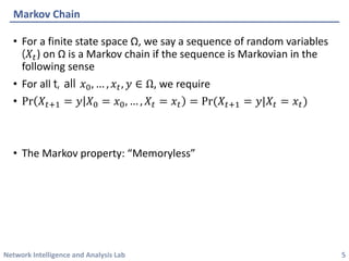
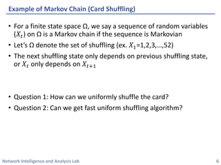
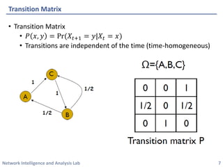
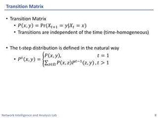
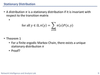
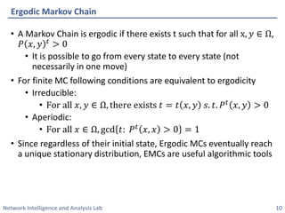
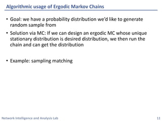
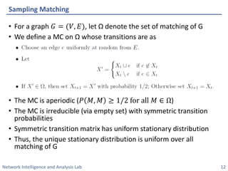
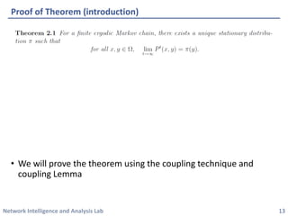
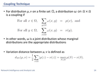
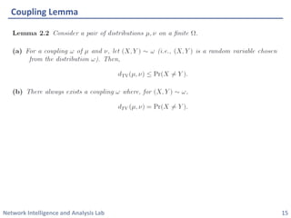
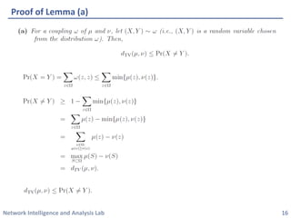
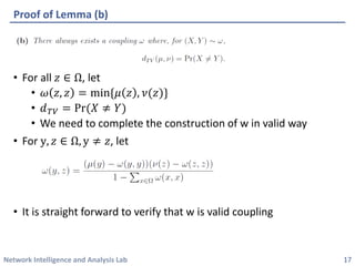
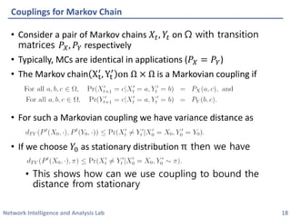
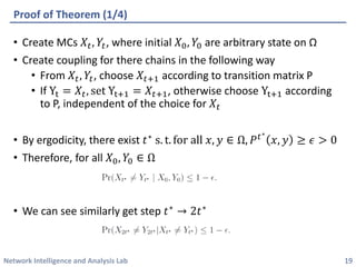
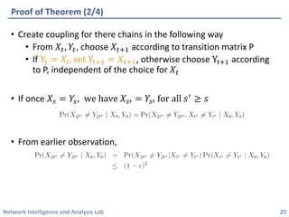
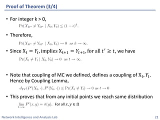
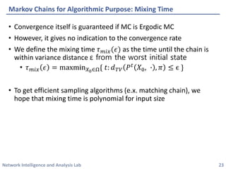
Network Intelligence and Analysis Lab
Markov Chain Basic
2014.07.11
SanghyukChun

•Exact Counting
•#P Complete
•Sampling and Counting
Previous Chapters
2

•Markov Chain Basic
•ErgodicMC has an unique stationary distribution
•Some basic concepts (Coupling, Mixing time)
•Coupling from past
•Coupling detail
•IsingModel
•Bounding Mixing time via Coupling
•Random spanning tree
•Path coupling framework
•MC for k-coloring graph
Remaining Chapters
3
Today!

•Introduce Markov Chain
•Show a potential algorithmic use of Markov Chain for sampling from complex distribution
•Prove that ErgodicMarkov Chain always converge to unique stationary distribution
•Introduce Coupling techniques and Mixing time
In this chapter…
4

•For a finite state space Ω, we say a sequence of random variables (푋푡) on Ωis a Markov chain if the sequence is Markovianin the following sense
•For all t, all 푥0,…,푥푡,푦∈Ω, we require
•Pr푋푡+1=푦푋0=푥0,…,푋푡=푥푡=Pr(푋푡+1=푦|푋푡=푥푡)
•The Markov property: “Memoryless”
Markov Chain
5

•For a finite state space Ω, we say a sequence of random variables (푋푡) on Ωis a Markov chain if the sequence is Markovian
•Let’s Ωdenote the set of shuffling (ex. 푋1=1,2,3,…,52)
•The next shuffling state only depends on previous shuffling state, or 푋푡only depends on 푋푡+1
•Question 1: How can we uniformly shuffle the card?
•Question 2: Can we get fast uniform shuffling algorithm?
Example of Markov Chain (Card Shuffling)
6

•Transition Matrix
•푃푥,푦=Pr(푋푡+1=푦|푋푡=푥)
•Transitions are independent of the time (time-homogeneous)
Transition Matrix
7

•Transition Matrix
•푃푥,푦=Pr(푋푡+1=푦|푋푡=푥)
•Transitions are independent of the time (time-homogeneous)
•The t-step distribution is defined in the natural way
•푃푡푥,푦= 푃푥,푦,푡=1 푧∈Ω푃푥,푧푃푡−1(푧,푦),푡>1
Transition Matrix
8

•A distribution 휋is a stationary distribution if it is invariant with respect to the transition matrix
• forall푦∈Ω,휋푦= 푥∈Ω 휋푥푃(푥,푦)
•Theorem 1
•For a finite ergodicMarkov Chain, there exists a unique stationary distribution 휋
•Proof?
Stationary Distribution
9

•A Markov Chain is ergodicif there exists t such that for all x,푦∈Ω, 푃푥,푦푡>0
•It is possible to go from every state to every state (not necessarily in one move)
•For finite MC following conditions are equivalent to ergodicity
•Irreducible:
•Forall푥,푦∈Ω,thereexists푡=푡푥,푦푠.푡.푃푡푥,푦>0
•Aperiodic:
•Forall푥∈Ω,gcd푡:푃푡푥,푥>0=1
•Since regardless of their initial state, ErgodicMCs eventually reach a unique stationary distribution, EMCs are useful algorithmic tools
ErgodicMarkov Chain
10

•Goal: we have a probability distribution we’d like to generate random sample from
•Solution via MC: If we can design an ergodicMC whose unique stationary distribution is desired distribution, we then run the chain and can get the distribution
•Example: sampling matching
Algorithmic usage of ErgodicMarkov Chains
11

•For a graph 퐺=(푉,퐸), let Ωdenote the set of matching of G
•We define a MC on Ωwhose transitions are as
•Choose an edge e uniformly at random from E
•Let, 푋′= 푋푡∪푒,if푒∉푋푡 푋푡푒,if푒∈푋푡
•If 푋′∈Ω, then set 푋푡+1=푋′with probability ½; otherwise set 푋푡+1=푋푡
•The MC is aperiodic (푃푀,푀≥1/2forall푀∈Ω)
•The MC is irreducible (via empty set) with symmetric transition probabilities
•Symmetric transition matrix has uniform stationary distribution
•Thus, the unique stationary distribution is uniform over all matching of G
Sampling Matching
12

•We will prove the theorem using the coupling technique and coupling Lemma
Proof of Theorem (introduction)
13

•For distribution 휇,휈on a finite setΩ, a distribution ωon Ω×Ωis a coupling if
•In other words, ωis a joint distribution whose marginal distributions are the appropriate distributions
•Variation distance between 휇,휈is defined as
Coupling Technique
14

Coupling Lemma
15

Proof of Lemma (a)
16

•For all 푧∈Ω, let
•휔푧,푧=min{휇푧,휈(푧)}
•푑푇푉=Pr(푋≠푌)
•We need to complete the construction of w in valid way
•For y,푧∈Ω,y≠푧, let
•It is straight forward to verify that w is valid coupling
Proof of Lemma (b)
17

•Consider a pair of Markov chains 푋푡,푌푡on Ωwith transition matrices 푃푋,푃푌respectively
•Typically, MCs are identical in applications (푃푋=푃푌)
•The Markov chainXt′ ,Yt′onΩ×Ωis a Markoviancoupling if
•For such a Markoviancoupling we have variance distance as
•If we choose 푌0as stationary distribution πthen we have
•This shows how can we use coupling to bound the distance from stationary
Couplings for Markov Chain
18

•Create MCs 푋푡,푌푡, where initial 푋0,푌0are arbitrary state on Ω
•Create coupling for there chains in the following way
•From 푋푡,푌푡, choose 푋푡+1according to transition matrix P
•If Yt=푋푡,setYt+1=푋푡+1, otherwise choose Yt+1according to P, independent of the choice for 푋푡
•By ergodicity, there exist 푡∗s.t.forall푥,푦∈Ω,푃푡∗ 푥,푦≥휖>0
•Therefore, for all 푋0,푌0∈Ω
•We can see similarly get step 푡∗→2푡∗
Proof of Theorem(1/4)
19

•Create coupling for there chains in the following way
•From 푋푡,푌푡, choose 푋푡+1according to transition matrix P
•If Yt=푋푡,setYt+1=푋푡+1, otherwise choose Yt+1according to P, independent of the choice for 푋푡
•If once 푋푠=푌푠,wehave푋푠′=푌푠′forall푠′≥푠
•From earlier observation,
20

•For integer k > 0,
•Therefore,
•Since Xt=푌푡,impliesXt+1=푌푡+1,forall푡′≥푡, we have
•Note that coupling of MC we defined, defines a coupling of Xt,푌푡. Hence by Coupling Lemma,
•This proves that from any initial points we reach same distribution
21
For all 푥,푦∈Ω

•From previous result, we proves there is a limiting distribution σ
•Question: is σa stationary distribution? Or satisfiesforall푦∈Ω,휎푦= 푥∈Ω 휎푥푃(푥,푦)
Proof of Theorem (4/4)
22

•Convergence itself is guaranteed if MC is ErgodicMC
•However, it gives no indication to the convergence rate
•We define the mixing time 휏푚푖푥(휖)as the time until the chain is within variance distance εfrom the worst initial state
•휏푚푖푥휖=maxmin푋0∈Ω{푡:푑푇푉푃푡푋0,∙,휋≤ϵ}
•To get efficient sampling algorithms (e.x. matching chain), we hope that mixing time is polynomial for input size
Markov Chains for Algorithmic Purpose: Mixing Time
23

Markov Chain Basic

More Related Content

What's hot

Viewers also liked

Similar to Markov Chain Basic

Recently uploaded

Markov Chain Basic