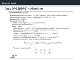
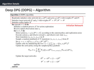
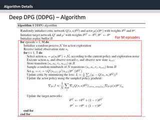
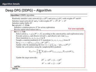
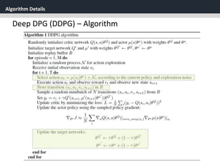
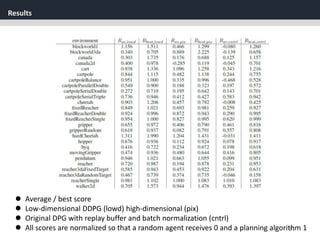
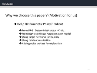
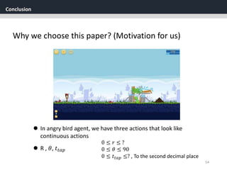
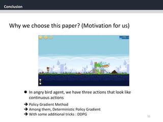
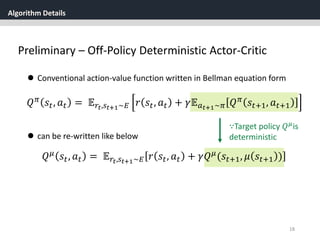
The document discusses the application of deep reinforcement learning with a focus on continuous control, specifically utilizing the Deep Deterministic Policy Gradient (DDPG) method. It addresses challenges in applying DQN to continuous action spaces and introduces techniques such as batch normalization, replay buffers, and exploration policies to improve learning stability and efficiency. Experimental results demonstrate the effectiveness of DDPG in high-dimensional state spaces, highlighting its performance improvements over traditional methods.

1. Continuous Control with Deep
Reinforcement Learning
Steve JobSae
Wangyu Han, Eunjoo Yang

2. Continuous Control with Deep Reinforcement Learning
2
1 Overview
3 Results
2 Algorithm Detail
4 Conclusion

3. Continuous Control with Deep Reinforcement Learning
3
1 Overview
3 Results
2 Algorithm Detail
4 Conclusion

4. Overview
4
Why we choose this paper?
 Angry Birds has
 High-dimensional state spaces
 3-dimensional continuous action spaces
 𝜃 (-90.00°~ 90.00°), R (𝑝𝑖𝑥𝑒𝑙), 𝑡𝑡𝑎𝑝 (𝑚𝑠)

5. Overview
5
Why we choose this paper? (Motivation for us)
 Policy Gradient
 Better convergence properties
 Effective in high-dimensional or continuous action spaces
 DQN
 Can solve problems with high-dimensional state spaces
 How about Policy Gradient Method + DQN?

6. Overview
6
Motivation for authors
 Trying to use DQN in continuous action domains
 However, DQN can only handle discrete and low-dimensional action
spaces
 To adapt DQN to continuous domains, action spaces should be discretized
 However, to apply fine-grained discretization, a number of discrete actions
will explode

7. Overview
7
Motivation for authors
 For example, in 7 degree of freedom system with rough discretization
𝑎𝑖 ∈ −𝑘, 0, 𝑘 , A number of actions will be 37
= 2187
 Such large action spaces are difficult to explore efficiently

8. Overview
8
How to solve the problem in this paper?
 Off-policy actor-critic algorithm with deep function approximator
DDPG = DQN + DPG
Deep
Deterministic
Policy
Gradient
 Use Policy Gradient Method
 Among them, Deterministic Policy Gradient

9. Continuous Control with Deep Reinforcement Learning
9
1 Overview
3 Results
2 Algorithm Detail
4 Conclusion

10. Algorithm Details
10
DDPG = DQN + DPG

11. Algorithm Details
11
 Unprocessed raw pixels were used for raw input
DQN for Continuous Action Space?

12. Algorithm Details
12
 It is not possible to straightforwardly apply Q-learning to continuous
action spaces
𝐿𝑖 𝜃𝑖 = 𝔼 𝑠,𝑎,𝑟,𝑠′ ~𝑈(𝐷) 𝑟 + 𝛾 max
𝑎′
𝑄 𝑠′
, 𝑎′
; 𝜃𝑖
−
− 𝑄 𝑠, 𝑎; 𝜃𝑖
2
Improper for Q continuous action
DQN for Continuous Action Space?

13. Algorithm Details
13
 It is not possible to straightforwardly apply Q-learning to continuous
action spaces
𝐿𝑖 𝜃𝑖 = 𝔼 𝑠,𝑎,𝑟,𝑠′ ~𝑈(𝐷) 𝑟 + 𝛾 max
𝑎′
𝑄 𝑠′
, 𝑎′
; 𝜃𝑖
−
− 𝑄 𝑠, 𝑎; 𝜃𝑖
2
 DPG maintains a parameterized actor function which specifies the
current policy by deterministically mapping states to a specific action
𝜇(𝑠|𝜃 𝜇)
 DDPG uses actor-critic approach based on the DPG algorithm
DQN for Continuous Action Space?

14. Algorithm Details
14
DDPG = DQN + DPG

15. Algorithm Details
15
Preliminary – DPG (Deterministic Policy Gradient)
 Deterministic Policy Gradient (presented by Pork BBQ team)
 Instead of using stochastic policy
𝜋 𝜃 𝑠, 𝑎 = 𝑝(𝑎|𝑠; 𝜃)

16. Algorithm Details
16
Preliminary – DPG (Deterministic Policy Gradient)
 Deterministic Policy Gradient (presented by Pork BBQ team)
 Instead of using stochastic policy
𝜋 𝜃 𝑠, 𝑎 = 𝑝(𝑎|𝑠; 𝜃)
 DPG defines policy as deterministic one
𝑎 = 𝜇 𝜃(𝑠)
𝜇 ∶ 𝑆 → 𝐴

17. Algorithm Details
17
Preliminary – Off-Policy Deterministic Actor-Critic
 Conventional action-value function written in Bellman equation form
𝑄 𝜋 𝑠𝑡, 𝑎 𝑡 = 𝔼 𝑟𝑡,𝑠 𝑡+1~𝐸 𝑟 𝑠𝑡, 𝑎 𝑡 + 𝛾𝔼 𝑎 𝑡+1~𝜋 𝑄 𝜋 𝑠𝑡+1, 𝑎 𝑡+1

18. Algorithm Details
18
Preliminary – Off-Policy Deterministic Actor-Critic
 Conventional action-value function written in Bellman equation form
𝑄 𝜋 𝑠𝑡, 𝑎 𝑡 = 𝔼 𝑟𝑡,𝑠 𝑡+1~𝐸 𝑟 𝑠𝑡, 𝑎 𝑡 + 𝛾𝔼 𝑎 𝑡+1~𝜋 𝑄 𝜋 𝑠𝑡+1, 𝑎 𝑡+1
 can be re-written like below
𝑄 𝜇
𝑠𝑡, 𝑎 𝑡 = 𝔼 𝑟𝑡,𝑠 𝑡+1~𝐸 𝑟 𝑠𝑡, 𝑎 𝑡 + 𝛾𝑄 𝜇
(𝑠𝑡+1, 𝜇 𝑠𝑡+1 )
∵Target policy 𝑄 𝜇is
deterministic

19. Algorithm Details
19
Preliminary – Off-Policy Deterministic Actor-Critic
 Critic : Q-Learning Off-policy Algorithm
 Linear function approximation parameterized by 𝜃 𝑄
 Minimize MSE between target Q from TD and approximated Q function
𝑦𝑡 = 𝑟 𝑠𝑡, 𝑎 𝑡 + 𝛾𝑄(𝑠𝑡+1, 𝜇 (𝑠𝑡+1)|𝜃 𝑄)
𝑤ℎ𝑒𝑟𝑒,
𝐿 𝜃 𝑄
= 𝔼 𝑠 𝑡~𝜌 𝛽,𝑎 𝑡~𝛽,𝑟𝑡~𝐸 𝑄 𝑠𝑡, 𝑎 𝑡 𝜃 𝑄
− 𝑦𝑡
2
Exploration by stochastic policy 𝛽

20. Algorithm Details
20
Preliminary – Off-Policy Deterministic Actor-Critic
 Actor : Deterministic Policy Gradient
 Update policy parameters 𝑄 𝜇
in the direction of action-value gradient
𝛻𝜃 𝜇 𝐽 ≈ 𝔼 𝑠 𝑡~𝜌 𝛽 𝛻𝜃 𝜇 𝑄 𝑠, 𝑎 𝜃 𝑄
𝑠=𝑠 𝑡,𝑎=𝜇 𝑠𝑡 𝜃 𝜇
= 𝔼 𝑠 𝑡~𝜌 𝛽 𝛻𝑎 𝑄 𝑠, 𝑎 𝜃 𝑄
𝑠=𝑠 𝑡,𝑎=𝜇 𝑠 𝑡
𝛻𝜃 𝜇
𝜇 𝑠 𝜃 𝜇
𝑠=𝑠 𝑡
By
chain
rule

21. Algorithm Details
21
DDPG
 Critic : Deep Q-Network
 Non-linear function approximation parameterized by 𝜃 𝑄
𝐿 𝜃 𝑄 = 𝔼 𝑠 𝑡~𝜌 𝛽,𝑎 𝑡~𝛽,𝑟𝑡~𝐸 𝑄 𝑠𝑡, 𝑎 𝑡 𝜃 𝑄 − 𝑦𝑡
2
𝑦𝑡 = 𝑟 𝑠𝑡, 𝑎 𝑡 + 𝛾𝑄′(𝑠𝑡+1, 𝜇′(𝑠𝑡+1|𝜃 𝜇′
)|𝜃 𝑄′
)
𝐿𝑖 𝜃𝑖 = 𝔼 𝑠,𝑎,𝑟,𝑠′ ~𝑈(𝐷) 𝑟 + 𝛾 max
𝑎′
𝑄 𝑠′
, 𝑎′
; 𝜃𝑖
−
− 𝑄 𝑠, 𝑎; 𝜃𝑖
2
 Original DQN

22. Algorithm Details
22
DDPG = DQN + DPG

23. Algorithm Details
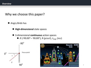
23
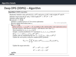
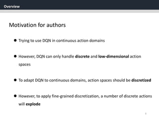
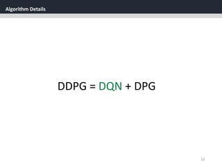
Deep DPG (DDPG)
[1] Replay Buffer
 One challenge when using neural networks for reinforcement
learning is that most optimization algorithms assume that the
samples are independently and identically distributed.
 When the samples are generated from exploring sequentially in
an environment this assumption no longer holds.

24. Algorithm Details
24
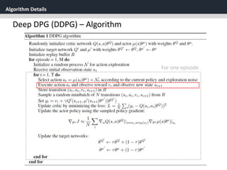
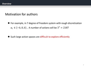
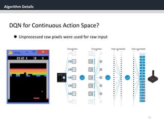
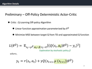
Deep DPG (DDPG)
[1] Replay Buffer
 One challenge when using neural networks for reinforcement
learning is that most optimization algorithms assume that the
samples are independently and identically distributed.
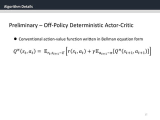
 When the samples are generated from exploring sequentially in
an environment this assumption no longer holds.
 Use Replay Buffer
- Replay buffer is a finite sized cache ℛ
- (𝑠𝑡, 𝑎 𝑡, 𝑟𝑡, 𝑠𝑡+1) are stored in the replay buffer
- At each time step the actor and critic are updated by sampling
a mini batch uniformly from the buffer.

25. Algorithm Details
25
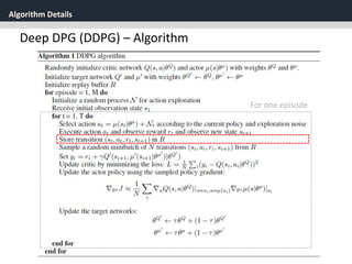
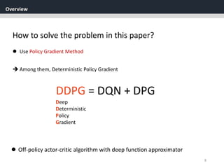
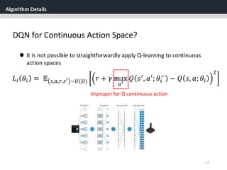
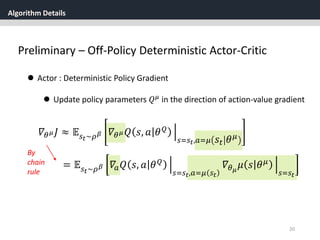
Deep DPG (DDPG)
[2] soft target updates
 Directly implementing Q learning with neural networks proved to
be unstable in many environments.
 Since the network being updated is also used in
calculating the target value, the Q update is prone to divergence.
𝑄(𝑠, 𝑎|𝜃 𝑄
)

26. Algorithm Details
26
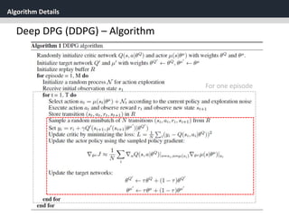
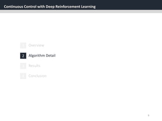
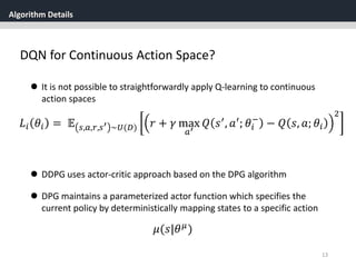
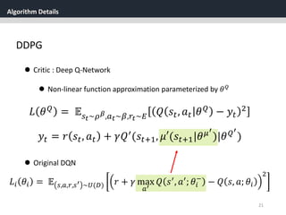
Deep DPG (DDPG)
[2] soft target updates
 Directly implementing Q learning with neural networks proved to
be unstable in many environments.
 Since the network being updated is also used in
calculating the target value, the Q update is prone to divergence.
𝑄(𝑠, 𝑎|𝜃 𝑄
)
 Soft Target updates,
rather than directly copying the weights.

27. Algorithm Details
27
Deep DPG (DDPG)
[2] soft target updates
 Creating a copy of the actor and critic networks respectively that
are used for calculating the target networks
𝑄′ 𝑠, 𝑎 𝜃 𝑄′
, 𝜇′(𝑠|𝜃 𝜇′
)

28. Algorithm Details
28
Deep DPG (DDPG)
[2] soft target updates
 Creating a copy of the actor and critic networks respectively that
are used for calculating the target networks
𝑄′ 𝑠, 𝑎 𝜃 𝑄′
, 𝜇′(𝑠|𝜃 𝜇′
)
 The weights of these target networks are then updated by having
them slowly track the learned networks:
𝜃′ ← 𝜏𝜃 + 1 − 𝜏 𝜃′ , 𝑤ℎ𝑒𝑟𝑒 𝜏 ≪ 1

29. Algorithm Details
29
Deep DPG (DDPG)
[2] soft target updates
 Creating a copy of the actor and critic networks respectively that
are used for calculating the target networks
𝑄′ 𝑠, 𝑎 𝜃 𝑄′
, 𝜇′(𝑠|𝜃 𝜇′
)
 The weights of these target networks are then updated by having
them slowly track the learned networks:
𝜃′ ← 𝜏𝜃 + 1 − 𝜏 𝜃′ , 𝑤ℎ𝑒𝑟𝑒 𝜏 ≪ 1
This means that the target values are constrained to change slowly, greatly
improving the stability of learning

30. Algorithm Details
30
Deep DPG (DDPG)
[3] batch normalization
 When learning from low dimensional feature vector observations,
the different components of the observation may have different
physical units (e.g., positions vs velocities) and the range may vary
across environments

31. Algorithm Details
31
Deep DPG (DDPG)
[3] batch normalization
 When learning from low dimensional feature vector observations,
the different components of the observation may have different
physical units (e.g., positions vs velocities) and the range may vary
across environments
 Using batch normalization

32. Algorithm Details
32
Deep DPG (DDPG)
[3] batch normalization
 When learning from low dimensional feature vector observations,
the different components of the observation may have different
physical units (e.g., positions vs velocities) and the range may vary
across environments
 Batch normalization technique normalizes each dimension across
the samples in a mini batch to have unit mean and variance.
 Using batch normalization
 DDPG uses batch normalization on the state input and all layers of
the 𝜇 network and all layers of the Q network prior to the action
input

33. Algorithm Details
33
Deep DPG (DDPG)
[4] exploration in continuous action space
 A major challenge of learning in continuous action spaces is
exploration

34. Algorithm Details
34
Deep DPG (DDPG)
[4] exploration in continuous action space
 A major challenge of learning in continuous action spaces is
exploration
 DDPG constructed an exploration policy 𝜇′ by adding noise
sampled from a noise process 𝒩 to the actor policy
𝜇′ 𝑠𝑡 = 𝜇 𝑠𝑡 𝜃𝑡
𝜇
+ 𝒩

35. Algorithm Details
35
Deep DPG (DDPG) – Algorithm

36. Algorithm Details
36
Deep DPG (DDPG) – Algorithm
Initialize Network

37. Algorithm Details
37
Deep DPG (DDPG) – Algorithm
For M episodes

38. Algorithm Details
38
Deep DPG (DDPG) – Algorithm
For one episode

39. Algorithm Details
39
Deep DPG (DDPG) – Algorithm
For one episode

40. Algorithm Details
40
Deep DPG (DDPG) – Algorithm
For one episode

41. Algorithm Details
41
Deep DPG (DDPG) – Algorithm
For one episode

42. Algorithm Details
42
Deep DPG (DDPG) – Algorithm
For one episode

43. Algorithm Details
43
Deep DPG (DDPG) – Algorithm

44. Continuous Control with Deep Reinforcement Learning
44
1 Overview
3 Results
2 Algorithm Detail
4 Conclusion

45. Results
45
Experiment Environment

46. Results
46
Experiment Environment

47. Results
47
Experiment Results
Original DPG with batch normalization
DPG with target network
DPG with target networks and batch normalization
DPG with target networks from pixel-only inputs

48. Results
48
Experiment Results
Original DPG with batch normalization
DPG with target network
DPG with target networks and batch normalization
DPG with target networks from pixel-only inputs
 Authors evaluated the policy periodically during training by testing
it without exploration noise.

49. Results
49
Experiment Results
Original DPG with batch normalization
DPG with target network
DPG with target networks and batch normalization
DPG with target networks from pixel-only inputs
 Authors evaluated the policy periodically during training by testing
it without exploration noise.
 Learning without a target network, as in the original work with DPG,
is very poor in many environments (light gray)

50. Results
50
Experiment Results
Original DPG with batch normalization
DPG with target network
DPG with target networks and batch normalization
DPG with target networks from pixel-only inputs
 In some simpler cases, learning policies from pixels is just as fast as
learning using the low-dimensional state descriptor

51. Results
51
 Average / best score
 Low-dimensional DDPG (lowd) high-dimensional (pix)
 Original DPG with replay buffer and batch normalization (cntrl)
 All scores are normalized so that a random agent receives 0 and a planning algorithm 1

52. Continuous Control with Deep Reinforcement Learning
52
1 Overview
3 Results
2 Algorithm Detail
4 Conclusion

53. Conclusion
53
Why we choose this paper? (Motivation for us)
From DPG : Deterministic Actor - Critic
From DQN : Nonlinear Approximation model
Using target networks for stability
Using batch normalization
Adding noise process for exploration
 Deep Deterministic Policy Gradient

54. Conclusion
54
Why we choose this paper? (Motivation for us)
 In angry bird agent, we have three actions that look like
continuous actions
 R , 𝜃, 𝑡𝑡𝑎𝑝
0 ≤ 𝑟 ≤ ?
0 ≤ 𝜃 ≤ 90
0 ≤ 𝑡𝑡𝑎𝑝 ≤? , To the second decimal place

55. Conclusion
55
Why we choose this paper? (Motivation for us)
 Policy Gradient Method
 Among them, Deterministic Policy Gradient
 With some additional tricks : DDPG
 In angry bird agent, we have three actions that look like
continuous actions

56. Thank you