The document discusses Bayesian Model-Agnostic Meta-Learning (BMAML) and its relationship with Model-Agnostic Meta-Learning (MAML), introducing techniques like Stein Variational Gradient Descent (SVGD) for improved performance. It presents a new meta-update method called 'chaser loss' to minimize the distance between task-training and true posteriors, which enhances performance in few-shot learning tasks. Empirical results demonstrate that BMAML outperforms traditional MAML methods in various applications, including regression, classification, and reinforcement learning.

1. Bayesian Model-Agnostic Meta-Learning
(NeurIPS 2018 spotlight)
2019.01.02.
Sangwoo Mo
1

2. Introduction
• Meta-Learning
• Learning is to find a model which works well for the given task 𝑇
• Meta-learning is to learn a “way to learn” a model when some task 𝑇𝑖 ∼ 𝑝(𝑇) is given
2

3. Introduction
• Meta-Learning
• Learning is to find a model which works well for the given task 𝑇
• Meta-learning is to learn a “way to learn” a model when some task 𝑇𝑖 ∼ 𝑝(𝑇) is given
• Example)
Learning: Train a CNN on ImageNet
Meta-learning: Learn a “way to learn” a model (e.g., network architecture, optimizer),
when some dataset (e.g., MNIST, CIFAR-10, SVHN) is given
3

4. Introduction
• Meta-Learning
• Learning is to find a model which works well for the given task 𝑇
• Meta-learning is to learn a “way to learn” a model when some task 𝑇𝑖 ∼ 𝑝(𝑇) is given
• Model-Agnostic Meta Learning (MAML)1
• Find a good initial point 𝜃, which can be easily adopted to 𝜃𝑖 for the task 𝑇𝑖
41. Finn et al. Model-Agnostic Meta-Learning for Fast Adaptation of Deep Networks. ICML 2017.
inner loop
outer loop

5. Background
• Bayesian Interpretation for MAML2
• MAML can be viewed as an hierarchical Bayesian model
with global variable 𝜃 and local variables 𝜙𝑗(= 𝜃𝑗)
52. Grant et al. Recasting Gradient-Based Meta-Learning as Hierarchical Bayes. ICLR 2018.

6. Background
• Bayesian Interpretation for MAML2
• MAML can be viewed as an hierarchical Bayesian model
with global variable 𝜃 and local variables 𝜙𝑗(= 𝜃𝑗)
• To compute marginal likelihood 𝑝 𝑋 𝜃 , one need to compute integral ∫ 𝑝(𝜙𝑗|𝜃)
62. Grant et al. Recasting Gradient-Based Meta-Learning as Hierarchical Bayes. ICLR 2018.

7. Background
• Bayesian Interpretation for MAML2
• MAML can be viewed as an hierarchical Bayesian model
with global variable 𝜃 and local variables 𝜙𝑗(= 𝜃𝑗)
• To compute marginal likelihood 𝑝 𝑋 𝜃 , one need to compute integral ∫ 𝑝(𝜙𝑗|𝜃)
• For example, using a point (MAP) estimate ෠𝜙𝑗 (computed by the inner loop)
recovers the original MAML objective
72. Grant et al. Recasting Gradient-Based Meta-Learning as Hierarchical Bayes. ICLR 2018.

8. Background
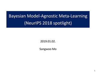
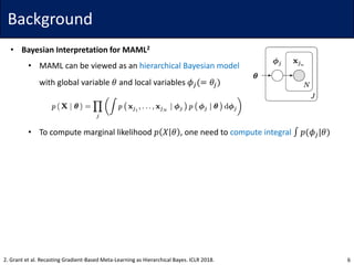
• Bayesian Interpretation for MAML2
• MAML can be viewed as an hierarchical Bayesian model
with global variable 𝜃 and local variables 𝜙𝑗(= 𝜃𝑗)
• To compute marginal likelihood 𝑝 𝑋 𝜃 , one need to compute integral ∫ 𝑝(𝜙𝑗|𝜃)
• For example, using a point (MAP) estimate ෠𝜙𝑗 (computed by the inner loop)
recovers the original MAML objective
• [2] propose to use a Laplace approximation
which allows to measure the uncertainty and improves the performance
82. Grant et al. Recasting Gradient-Based Meta-Learning as Hierarchical Bayes. ICLR 2018.

9. Background
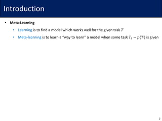
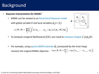
• Bayesian Interpretation for MAML2
• [2] propose to use a Laplace approximation
which allows to measure the uncertainty and improves the performance
92. Grant et al. Recasting Gradient-Based Meta-Learning as Hierarchical Bayes. ICLR 2018.

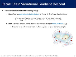
10. Method
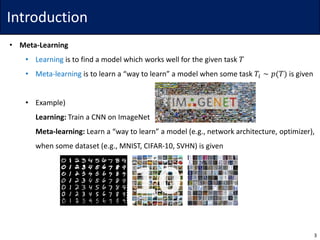
• Bayesian Model-Agnostic Meta-Learning (BMAML)3
• Can one extend [2] to more complex Bayesian neural network?
• Instead of approximating 𝑝(𝜙𝑗|𝜃) with tractable form, simply sampling from
• Here, the sampled 𝜙𝑗s should be differentiable
103. Kim et al. Bayesian Model-Agnostic Meta-Learning. NeurIPS 2018.

11. Method
• Bayesian Model-Agnostic Meta-Learning (BMAML)3
• Can one extend [2] to more complex Bayesian neural network?
• Instead of approximating 𝑝(𝜙𝑗|𝜃) with tractable form, simply sampling from
• Here, the sampled 𝜙𝑗s should be differentiable
• Idea: Use Stein Variational Gradient Descent (SVGD)*
11
3. Kim et al. Bayesian Model-Agnostic Meta-Learning. NeurIPS 2018.
* One can use any gradient-based MCMC algorithms (e.g., SGLD or SGHMC), but SVGD is deterministic and adapt faster.

12. Recall: Stein Variational Gradient Descent
• Stein Variational Gradient Descent (SVGD)4
• Goal: Find an approximated distribution 𝑞∗ (s.t. 𝑞 ∈ 𝒬) of true distribution 𝑝
124. Liu et al. Stein Variational Gradient Descent: A General Purpose Bayesian Inference Algorithm. NeurIPS 2016.

13. Recall: Stein Variational Gradient Descent
• Stein Variational Gradient Descent (SVGD)4
• Goal: Find an approximated distribution 𝑞∗ (s.t. 𝑞 ∈ 𝒬) of true distribution 𝑝
• Idea: Define 𝑞 by as a kernel density estimation (KDE) of finite particles {𝑥𝑖}
• One may need only samples from 𝑞∗
. Then {𝑥𝑖} can be good & diverse samples
134. Liu et al. Stein Variational Gradient Descent: A General Purpose Bayesian Inference Algorithm. NeurIPS 2016.

14. Recall: Stein Variational Gradient Descent
• Stein Variational Gradient Descent (SVGD)4
• Goal: Find an approximated distribution 𝑞∗ (s.t. 𝑞 ∈ 𝒬) of true distribution 𝑝
• Idea: Define 𝑞 by as a kernel density estimation (KDE) of finite particles {𝑥𝑖}
• One may need only samples from 𝑞∗
. Then {𝑥𝑖} can be good & diverse samples
• Algorithm:
1) Move particles toward high prob. regions
2) Diversify particles to evade mode collapse
144. Liu et al. Stein Variational Gradient Descent: A General Purpose Bayesian Inference Algorithm. NeurIPS 2016.

15. Recall: Stein Variational Gradient Descent
• Stein Variational Gradient Descent (SVGD)4
• Goal: Find an approximated distribution 𝑞∗ (s.t. 𝑞 ∈ 𝒬) of true distribution 𝑝
• Idea: Define 𝑞 by as a kernel density estimation (KDE) of finite particles {𝑥𝑖}
• One may need only samples from 𝑞∗
. Then {𝑥𝑖} can be good & diverse samples
• Algorithm:
1) Move particles toward high prob. regions
2) Diversify particles to evade mode collapse
• Cf. It is the steepest gradient direction (of KL div.) in the unit ball of a RKHS
(derivate of KL in RKHS = kernelized Stein discrepancy (KSD), hence named SVGD)
154. Liu et al. Stein Variational Gradient Descent: A General Purpose Bayesian Inference Algorithm. NeurIPS 2016.

16. Method
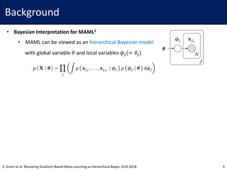
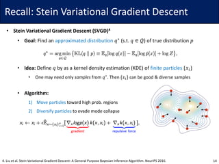
• Bayesian Model-Agnostic Meta-Learning (BMAML)3
• Can one extend [2] to more complex Bayesian neural network?
• Instead of approximating 𝑝(𝜙𝑗|𝜃) with tractable form, simply sampling from
• Idea: Use Stein Variational Gradient Descent (SVGD)
• Learn a task-specific posterior Θ 𝜏 with SVGD (start from the prior Θ0)*
• Meta-update for Θ0 is given by the mean of val. likelihoods of 𝑀 particles
• Cf. To reduce complexity, all particles share parameters all but the last linear layer
16
3. Kim et al. Bayesian Model-Agnostic Meta-Learning. NeurIPS 2018.
* Both Θ0 and Θ 𝜏 are given by 𝑀 particles.

17. Method
• Bayesian Model-Agnostic Meta-Learning (BMAML)3
• Can one extend [2] to more complex Bayesian neural network?
• Idea 1: Use Stein Variational Gradient Descent (SVGD)
• Learn a task-specific posterior Θ 𝜏 with SVGD (start from the prior Θ0)
• Meta-update for Θ0 is given by the mean of val. likelihoods of 𝑀 particles
• However, this meta-update it not Bayesian inference
• Same as MAML, minimizes empirical loss on task-validation sets (but ensembled)
• It is numerically unstable (task-validation likelihoods) and easily overfitted
173. Kim et al. Bayesian Model-Agnostic Meta-Learning. NeurIPS 2018.

18. Method
• Bayesian Model-Agnostic Meta-Learning (BMAML)3
• Can one extend [2] to more complex Bayesian neural network?
• Idea 1: Use Stein Variational Gradient Descent (SVGD)
• Learn a task-specific posterior Θ 𝜏 with SVGD (start from the prior Θ0)
• Meta-update for Θ0 is given by the mean of val. likelihoods of 𝑀 particles
• However, this meta-update it not Bayesian inference
• Same as MAML, minimizes empirical loss on task-validation sets (but ensembled)
• It is numerically unstable (task-validation likelihoods) and easily overfitted
• Instead, [3] propose a new meta-update algorithm in Bayesian scheme
183. Kim et al. Bayesian Model-Agnostic Meta-Learning. NeurIPS 2018.

19. Method
• Bayesian Model-Agnostic Meta-Learning (BMAML)3
• Can one extend [2] to more complex Bayesian neural network?
• Idea 1: Use Stein Variational Gradient Descent (SVGD)
• Idea 2: New meta-update algorithm (coined chaser loss) for Bayesian setting
• Directly minimize the distance between task-train posterior 𝑝𝜏
𝑛
and true posterior 𝑝𝜏
∞
193. Kim et al. Bayesian Model-Agnostic Meta-Learning. NeurIPS 2018.

20. Method
• Bayesian Model-Agnostic Meta-Learning (BMAML)3
• Can one extend [2] to more complex Bayesian neural network?
• Idea 1: Use Stein Variational Gradient Descent (SVGD)
• Idea 2: New meta-update algorithm (coined chaser loss) for Bayesian setting
• Directly minimize the distance between task-train posterior 𝑝𝜏
𝑛
and true posterior 𝑝𝜏
∞
• However, the problem is that one does not know the true posterior 𝑝𝜏
∞
203. Kim et al. Bayesian Model-Agnostic Meta-Learning. NeurIPS 2018.

21. Method
• Bayesian Model-Agnostic Meta-Learning (BMAML)3
• Can one extend [2] to more complex Bayesian neural network?
• Idea 1: Use Stein Variational Gradient Descent (SVGD)
• Idea 2: New meta-update algorithm (coined chaser loss) for Bayesian setting
• Directly minimize the distance between task-train posterior 𝑝𝜏
𝑛
and true posterior 𝑝𝜏
∞
• However, the problem is that one does not know the true posterior 𝑝𝜏
∞
• Hence, [3] approximates 𝑝𝜏
∞
with 𝑝𝜏
𝑛+𝑠
, updated by both task-train & task-validation data
• Here, 𝑝𝜏
𝑛+𝑠
(both train & val) is the leader, and 𝑝𝜏
𝑛
(train only) is the chaser
213. Kim et al. Bayesian Model-Agnostic Meta-Learning. NeurIPS 2018.

22. Method
• Bayesian Model-Agnostic Meta-Learning (BMAML)3
• Can one extend [2] to more complex Bayesian neural network?
• Idea 1: Use Stein Variational Gradient Descent (SVGD)
• Idea 2: New meta-update algorithm (coined chaser loss) for Bayesian setting
• Directly minimize the distance between task-train posterior 𝑝𝜏
𝑛
and true posterior 𝑝𝜏
∞
• [3] approximates 𝑝𝜏
∞
with 𝑝𝜏
𝑛+𝑠
, updated by both task-train & task-validation data
• Q. How to compute the distance between 𝑝𝜏
𝑛+𝑠
and 𝑝𝜏
𝑛
?
223. Kim et al. Bayesian Model-Agnostic Meta-Learning. NeurIPS 2018.

23. Method
• Bayesian Model-Agnostic Meta-Learning (BMAML)3
• Can one extend [2] to more complex Bayesian neural network?
• Idea 1: Use Stein Variational Gradient Descent (SVGD)
• Idea 2: New meta-update algorithm (coined chaser loss) for Bayesian setting
• Directly minimize the distance between task-train posterior 𝑝𝜏
𝑛
and true posterior 𝑝𝜏
∞
• [3] approximates 𝑝𝜏
∞
with 𝑝𝜏
𝑛+𝑠
, updated by both task-train & task-validation data
• Q. How to compute the distance between 𝑝𝜏
𝑛+𝑠
and 𝑝𝜏
𝑛
?
• Since both posteriors are given by finite particles, one can simply find a one-to-one
mapping, and minimize the pairwise 𝑙2 distance
233. Kim et al. Bayesian Model-Agnostic Meta-Learning. NeurIPS 2018.

24. Method
• Bayesian Model-Agnostic Meta-Learning (BMAML)3
• Can one extend [2] to more complex Bayesian neural network?
• Idea 1: Use Stein Variational Gradient Descent (SVGD)
• Idea 2: New meta-update algorithm (coined chaser loss) for Bayesian setting
• [3] approximates 𝑝𝜏
∞
with 𝑝𝜏
𝑛+𝑠
, updated by both task-train & task-validation data
• For posterior distance, simply minimize the pairwise 𝑙2 distance
243. Kim et al. Bayesian Model-Agnostic Meta-Learning. NeurIPS 2018.

25. Experiments
• Evaluate performance on various few-shot learning tasks
• E.g., regression, classification, active learning, reinforcement learning
• Compare with MAML and ensemble of MAML (EMAML)
25

26. Experiments
• Evaluate performance on various few-shot learning tasks
• E.g., regression, classification, active learning, reinforcement learning
• Compare with MAML and ensemble of MAML (EMAML)
• BMAML shows better performance, stability, and exploration
• Results in (synthetic) sinusoidal regression tasks
26

27. Experiments
• Evaluate performance on various few-shot learning tasks
• E.g., regression, classification, active learning, reinforcement learning
• Compare with MAML and ensemble of MAML (EMAML)
• BMAML shows better performance, stability, and exploration
• Results in image classification & active learning tasks
27

28. Experiments
• BMAML shows better performance, stability, and exploration
• Results in reinforcement learning
28

29. Conclusion
• MAML can be interpreted as an hierarchical Bayesian model
• BMAML propose two ideas
1) Use SVGD for the inner loop of algorithm
2) New meta-update (outer loop) algorithm (chaser loss)
• which shows better performance, stability, and explorations results
29