Downloaded 123 times

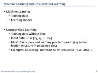
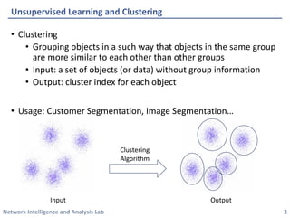
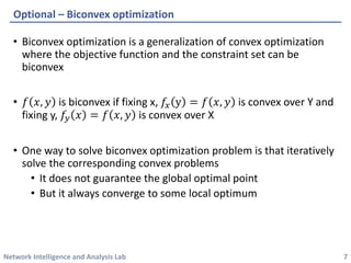
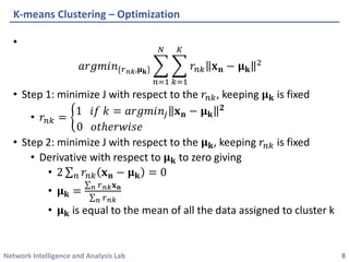
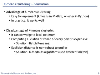
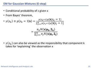
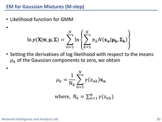
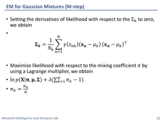
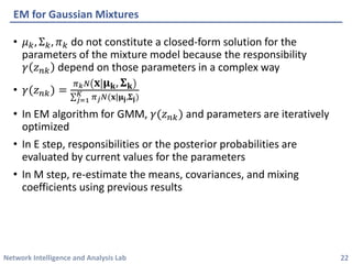

This document discusses clustering methods using the EM algorithm. It begins with an overview of machine learning and unsupervised learning. It then describes clustering, k-means clustering, and how k-means can be formulated as an optimization of a biconvex objective function solved via an iterative EM algorithm. The document goes on to describe mixture models and how the EM algorithm can be used to estimate the parameters of a Gaussian mixture model (GMM) via maximum likelihood.


![[토크아이티] 프런트엔드 개발 시작하기 저자 특강](https://cdn.slidesharecdn.com/ss_thumbnails/random-141024103422-conversion-gate01-thumbnail.jpg?width=640&height=640&fit=bounds)