This document presents a model-free, off-policy actor-critic algorithm to learn policies in continuous action spaces using deep reinforcement learning. The algorithm is based on deterministic policy gradients and extends DQN to continuous action domains by using deep neural networks to approximate the actor and critic. Challenges addressed include ensuring samples are i.i.d. by using a replay buffer, stabilizing learning with a target network, normalizing observations with batch normalization, and exploring efficiently with an Ornstein-Uhlenbeck process. The algorithm is able to learn policies on high-dimensional continuous control tasks.

1. Continuous control with deep
reinforcement learning
2016-06-28
Taehoon Kim

2. Motivation
• DQN can only handle
• discrete (not continuous)
• low-dimensional action spaces
• Simple approach to adapt DQN to continuous domain is discretizing
• 7 degree of freedom system with discretization 𝑎" ∈ {−𝑘, 0, 𝑘}
• Now space dimensionality becomes 3+
= 2187
• explosion of the number of discrete actions
2

3. Contribution
• Present a model-free, off-policy actor-critic algorithm
• learn policies in high-dimensional, continuous action spaces
• Work based on DPG (Deterministic policy gradient)
3

4. Background
• actions 𝑎" ∈ ℝ2
, action space 𝒜 = ℝ2
• history of observation, action pairs 𝑠" = (𝑥7, 𝑎7, … , 𝑎"97, 𝑥")
• assume fully-observable so 𝑠" = 𝑥"
• policy 𝜋: 𝒮 → 𝒫(𝒜)
• Model environment as Markov decision process
• initial state distribution 𝑝(𝑠7)
• transition dynamics 𝑝(𝑠"A7|𝑠", 𝑎")
4

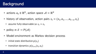
5. Background
• Discounted future reward 𝑅" = ∑ 𝛾F9"
𝑟(𝑠F, 𝑎F)H
FI"
• Goal of RL is to learn a policy 𝜋 which maximizes the expected return
• from the start distribution 𝐽 = 𝔼LM ,NM~P,QM~R[𝑅7]
• Discounted state visitation distribution for a policy 𝜋: ρR
5

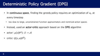
6. Background
• action-value function 𝑄R
𝑠", 𝑎" = 𝔼LMW",NMXY~P,QMXY~R[𝑅"|𝑠", 𝑎"]
• expected return after taking an action 𝑎" in state 𝑠" and following policy 𝜋
• Bellman equation
• 𝑄R
𝑠", 𝑎" = 𝔼LY,NYZ[~P[𝑟 𝑠", 𝑎" + 𝛾𝔼QYZ[~R 𝑄R
(𝑠"A7, 𝑎"A7) ]
• With deterministic policy 𝜇: 𝒮 → 𝒜
• 𝑄^
𝑠", 𝑎" = 𝔼LY,NYZ[~P[𝑟 𝑠", 𝑎" + 𝛾𝑄^
𝑠"A7, 𝜇(𝑠"A7 )]
6

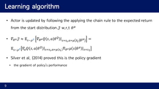
7. Background
• Expectation only depends on the environment
• possible to learn 𝑄 𝝁
off-policy, where transitions are generated from
different stochastic policy 𝜷
• Q-learning with greedy policy 𝜇 𝑠 = arg max
f
𝑄 𝑠, 𝑎
• 𝐿 𝜃i
= 𝔼NY~jk,QY~l,NY~P[ 𝑄 𝑠", 𝑎" 𝜃i
− 𝑦"
n
]
• where 𝑦" = 𝑟 𝑠", 𝑎" + 𝛾𝑄(𝑠"A7, 𝜇(𝑠"A7)|𝜃i
)
• To scale Q-learning into large non-linear approximators:
• a replay buffer, a separate target network
7
(a commonly used off-policy algorithm)

8. Deterministic Policy Gradient (DPG)
• In continuous space, finding the greedy policy requires an optimization of 𝑎" at
every timestep
• too slow to large, unconstrained function approximators and nontrivial action spaces
• Instead, used an actor-critic approach based on the DPG algorithm
• actor: 𝜇 𝑠 𝜃^
: 𝒮 → 𝒜
• critic: 𝑄(𝑠, 𝑎|𝜃i
)
8

9. Learning algorithm
• Actor is updated by following the applying the chain rule to the expected return
from the start distribution 𝒥 w.r.t 𝜃^
• 𝛻rs 𝒥 ≈ 𝔼N~j 𝜷 𝛻rs 𝑄 𝑠, 𝑎 𝜃i |NINY,QI^ 𝑠" 𝜃^ =
𝔼N~j 𝜷 𝛻Q 𝑄 𝑠, 𝑎 𝜃i |NINY,QI^ NY
∇rs 𝜇 𝑠 𝜃^ |NIN"
• Silver et al. (2014) proved this is the policy gradient
• the gradient of policy’s performance
9

10. Contributions
• Introducing non-linear function approximators means that
convergence is no longer guaranteed
• But essential to learn and generalize on large state spaces
• Contribution
• To provide modifications to DPG, inspired by the success of DQN
• Allow to use neural network function approximators to learn in large state and
action spaces online
10

11. Challenges 1
• NN for RL usually assume that the samples are i.i.d.
• but when the samples are generated from exploring sequentially in an environment,
this assumption no longer holds.
• As DQN, we use replay buffer to address this issue
• As DQN, we used target network for stable learning but use “soft” target
updates
• 𝜃` ← 𝜏𝜃 + 1 − 𝜏 𝜃`, with 𝜏 ≪ 1
• Target network slowly change that greatly improve the stability of learning
11

12. Challenges 2
• When learning from low dimensional feature vector, observations may have
different physical units (i.e. positions and velocities)
• make it difficult to learn effectively and also to find hyper-parameters which generalize across
environments
• Use batch normalization [Ioffe & Szegedy, 2015] to normalize each dimension
across the samples in a minibatch to have unit mean and variance
• Also maintains a running average of the mean and variance for normalization during testing
• Use all layers of 𝜇 and 𝑄 prior to the action input
• Can train different units without needing to manually ensure the units were within a set range
12
(exploration or evaluation)

13. Challenges 3
• Advantage of off-policies algorithm (i.e. DDPG) is that we can treat the problem
of exploration independently from the learning algorithm
• Constructed an exploration policy 𝜇` by adding noise sampled from a noise
process 𝒩
• 𝜇` 𝑠" = 𝜇 𝑠" 𝜃"
^
+ 𝒩
• Use an Ornstein-Uhlenbeck process to generate temporally
correlated exploration for exploration efficiency with inertia
13

14. 14

15. Experiment details
• Adam. 𝑙𝑟^
= 109|
, 𝑙𝑟i
= 109}
• 𝑄 include 𝐿n weight decay of 109n
and 𝛾 = 0.99
• 𝜏 = 0.001
• ReLU for hidden layers, tanh for output layer of the actor to bound the actions
• NN: 2 hidden layers with 400 and 300 units
• Action is not included until the 2nd hidden layer of 𝑄
• The final layer weights and biases are initialized from a uniform distribution −3×109}
,3×109}
• to ensure the initial outputs for the policy and value estimates were near zero
• The other layers are initialized from uniform distributions −
7
•
,
7
•
where 𝑓 is the fan-in of the layer
• Replay buffer ℛ = 10„
, Ornstein-Uhlenbeck process: 𝜃 = 0.15, 𝜎 = 0.2
15

16. References
1. [Wang, 2015] Wang, Z., de Freitas, N., & Lanctot, M. (2015). Dueling network architectures for
deep reinforcement learning. arXiv preprint arXiv:1511.06581.
2. [Van, 2015] Van Hasselt, H., Guez, A., & Silver, D. (2015). Deep reinforcement learning with
double Q-learning. CoRR, abs/1509.06461.
3. [Schaul, 2015] Schaul, T., Quan, J., Antonoglou, I., & Silver, D. (2015). Prioritized experience
replay. arXiv preprint arXiv:1511.05952.
4. [Sutton, 1998] Sutton, R. S., & Barto, A. G. (1998). Reinforcement learning: An introduction(Vol.
1, No. 1). Cambridge: MIT press.
16