Download as PDF, PPTX


![Matrix Exponential Method
• Our previous attempt [Weng12]
where
8](https://image.slidesharecdn.com/dac15zhuanghv15-150612224625-lva1-app6892/75/SPICE-MATEX-DAC15-8-2048.jpg)
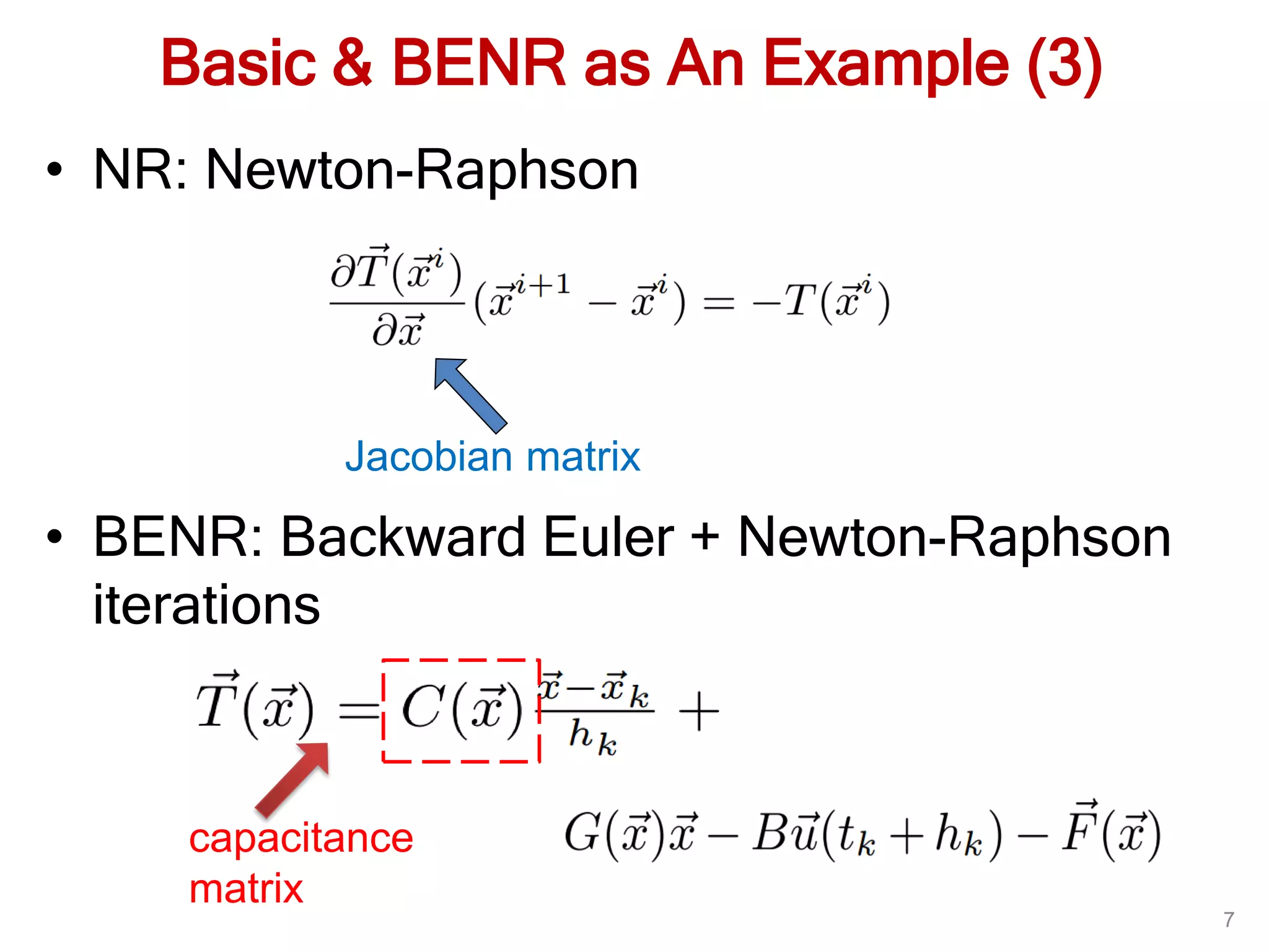
![Matrix Exponential Method
• Our previous attempt [Weng12]
where
• It also uses NR
The Jacobian matrix
9
capacitance matrix](https://image.slidesharecdn.com/dac15zhuanghv15-150612224625-lva1-app6892/75/SPICE-MATEX-DAC15-9-2048.jpg)
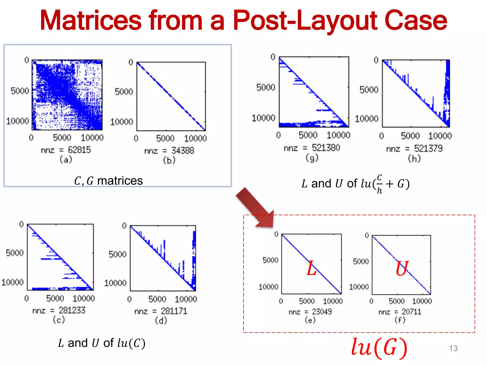
![10
𝐶, 𝐺 matrices from FreeCPU [Zhang, Yu TCAD 2013]
nnz: non-zero terms
𝐺𝐶
Matrices from a Post-Layout Case](https://image.slidesharecdn.com/dac15zhuanghv15-150612224625-lva1-app6892/75/SPICE-MATEX-DAC15-10-2048.jpg)


![ER: Exponential Rosenbrock
Start from
𝑑𝑥 𝑡
𝑑𝑡
= 𝑔(𝑥, 𝑢, 𝑡)
• The next time step solution [Hochbruck, et. al. SIAM09]
𝑥 𝑘+1 = 𝑥 𝑘 + 𝑘 𝜙1 𝑘 𝐽 𝑘 𝑔(𝑥 𝑘, 𝑢, 𝑡 𝑘) + 𝑘
2
𝜙2 𝑘 𝐽 𝑘 𝑏k
where 𝐽 𝑘 = 𝜕𝑔/𝜕𝑥, 𝑏 𝑘 = 𝜕𝑔/𝜕𝑡
𝜙1 𝑘 𝐽 𝑘 = (𝑒ℎ 𝑘 𝐽 𝑘−𝐼 𝑛)/ 𝑘 𝐽 𝑘
𝜙2 𝑘 𝐽 𝑘 = (𝑒ℎ 𝑘 𝐽 𝑘−𝐼 𝑛)/ 𝑘
2
𝐽 𝑘
2
− 𝐼 𝑛/ 𝑘 𝐽 𝑘
16
Exponential Integrators:
Proved to be Stable, Explicit, High-Order Accuracy for ODE](https://image.slidesharecdn.com/dac15zhuanghv15-150612224625-lva1-app6892/75/SPICE-MATEX-DAC15-16-2048.jpg)

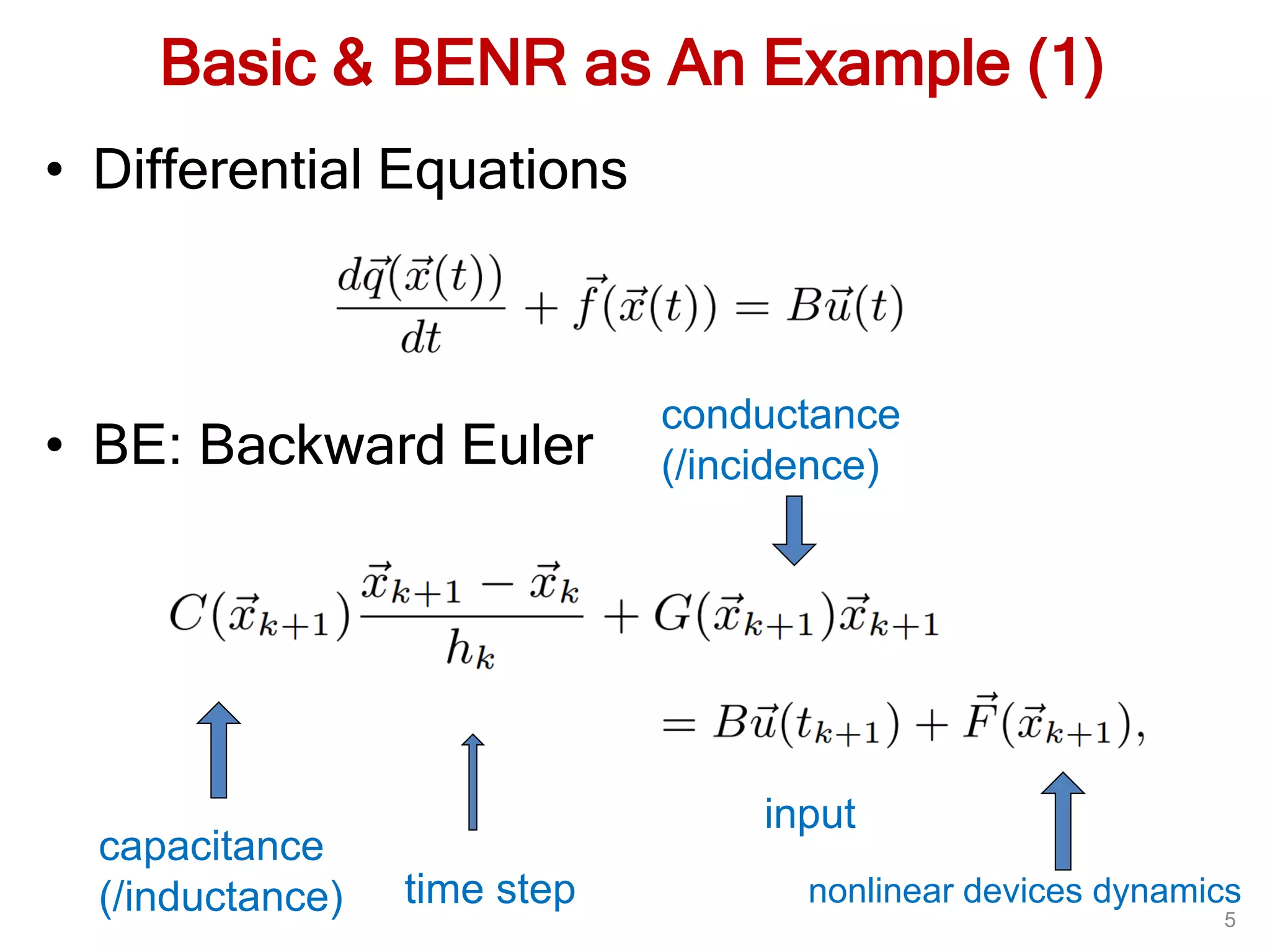
![Local Nonlinear Error Control
The local nonlinear error estimator [Caliari09]
𝑒 𝑟𝑟 𝑥 𝑘+1, 𝑥 𝑘 = 𝜙1 𝑘 𝐽 𝑘 𝐶 𝑘
−1
Δ𝐹𝑘
where Δ𝐹𝑘 = 𝐹 𝑥 𝑘+1 − 𝐹(𝑥 𝑘)
18
ER-C: ER with Correction Term
Reuse Δ𝐹𝑘 to improve the accuracy by padding
the extra term
𝐷 𝑘 = 𝛾 𝑘 𝜙2 𝑘 𝐽 𝑘 𝐶 𝑘
−1
Δ𝐹𝑘
The further corrected solution is
𝑥 𝑘+1,𝑐 = 𝑥 𝑘+1 − 𝐷 𝑘](https://image.slidesharecdn.com/dac15zhuanghv15-150612224625-lva1-app6892/75/SPICE-MATEX-DAC15-18-2048.jpg)
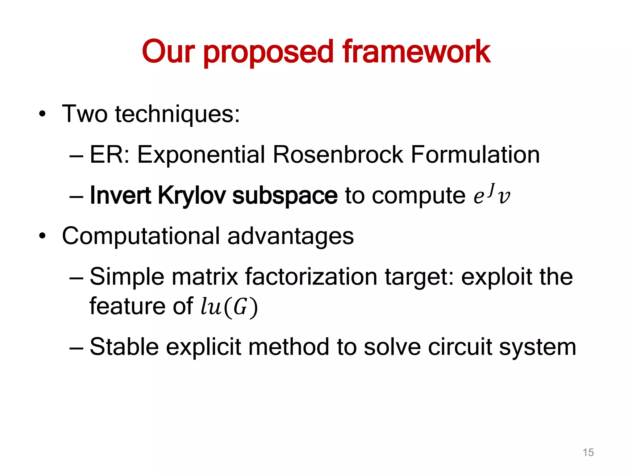
![Krylov Method for MEVP 𝑒 𝐽
𝑣
• 𝑒 𝐽 𝑣: Matrix Exponential and Vector Product
(MEVP) via standard Krylov subspace [Weng12]
𝐾 𝑚 𝐽, 𝑣 ≔ 𝑠𝑝𝑎𝑛 𝑣, 𝐽𝑣, 𝐽2 𝑣, … , 𝐽 𝑚−1 𝑣
– Arnoldi process and Matrix reduction:
𝐽𝑉𝑚 = 𝑉𝑚 𝐻 𝑚 + 𝑚+1,𝑚 𝑣 𝑚+1 𝑒 𝑚
T
• MEVP is computed by
𝑒 𝐽 𝑣 ≈ 𝑣 2 𝑉𝑚 𝑒 𝐻 𝑚 𝑒1
• Explicit feature: time stepping only by scaling 𝐻 𝑚
with h,
𝑒ℎ𝐽 𝑣 ≈ 𝑣 2 𝑉𝑚 𝑒ℎ𝐻 𝑚 𝑒1
19](https://image.slidesharecdn.com/dac15zhuanghv15-150612224625-lva1-app6892/75/SPICE-MATEX-DAC15-19-2048.jpg)
![20
Standard Krylov subspace
Im
Re0
“like” these eigenvalues
Eigenvalues of J: small magnitude of Re
Eigenvalues of J: large magnitude of Re
(a) Standard Krylov Basis [Weng12]
𝐾 𝑚 𝐽, 𝑣 ≔ 𝑠𝑝𝑎𝑛 𝑣, 𝐽𝑣, 𝐽2
𝑣, … , 𝐽 𝑚−1
𝑣
spectrum of
𝐽 = −𝑪−𝟏
𝑮](https://image.slidesharecdn.com/dac15zhuanghv15-150612224625-lva1-app6892/75/SPICE-MATEX-DAC15-20-2048.jpg)
![21
Standard Krylov subspace
Im
Re0
• these eigenvalues
defines the major
dynamical behavior
• demand more bases to
characterize
Eigenvalues of J: small magnitude of Re
Eigenvalues of J: large magnitude of Re
(a) Standard Krylov Basis [Weng12]
𝐾 𝑚 𝐽, 𝑣 ≔ 𝑠𝑝𝑎𝑛 𝑣, 𝐽𝑣, 𝐽2
𝑣, … , 𝐽 𝑚−1
𝑣
spectrum of
𝐽 = −𝑪−𝟏
𝑮](https://image.slidesharecdn.com/dac15zhuanghv15-150612224625-lva1-app6892/75/SPICE-MATEX-DAC15-21-2048.jpg)
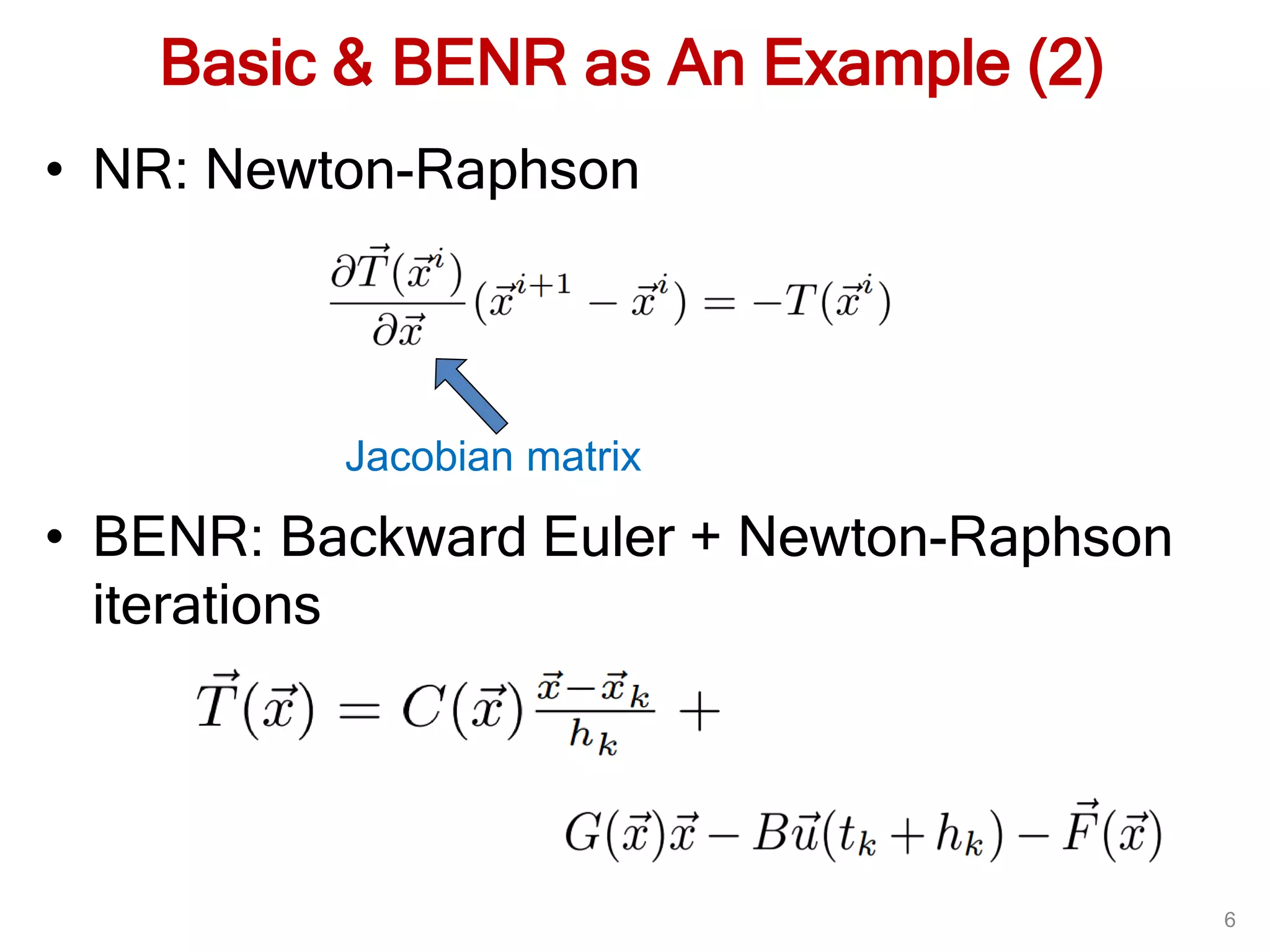
![22
Im
Re
Im
Re00
Invert Krylov subspace method captures
“important” eigenvalues in the original spectrum
Eigenvalues of J: small magnitude of Re
Eigenvalues of J: large magnitude of Re
Invert Krylov subspace
Invert Krylov Basis [Zhuang, et. al. DAC14]
𝐾 𝑚 𝐽−1, 𝑣 ≔ 𝑠𝑝𝑎𝑛 𝑣, 𝐽−1 𝑣, 𝐽−2 𝑣, … , 𝐽−𝑚+1 𝑣
spectrum of 𝐽−1
spectrum of 𝐽](https://image.slidesharecdn.com/dac15zhuanghv15-150612224625-lva1-app6892/75/SPICE-MATEX-DAC15-22-2048.jpg)

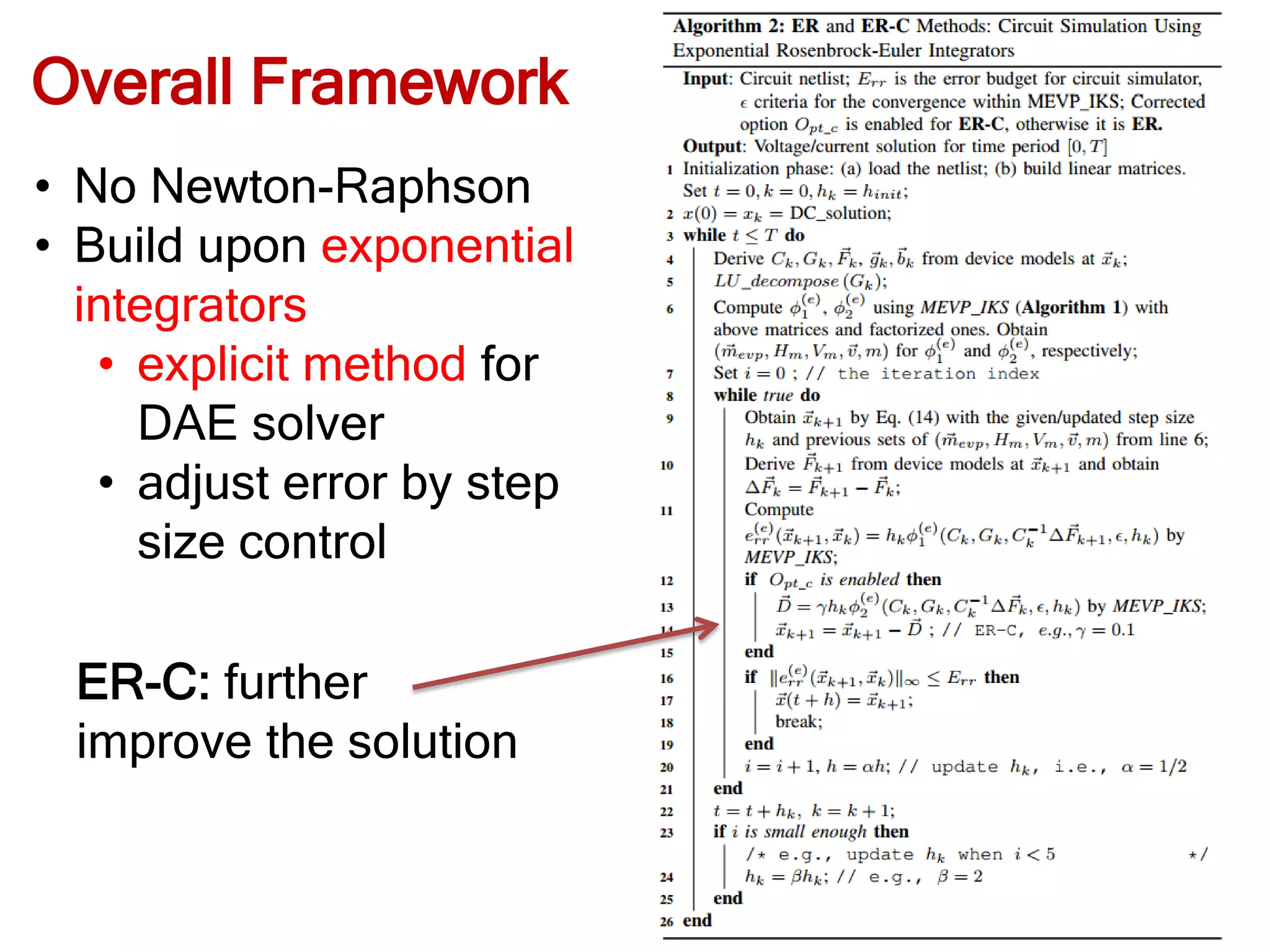


1. The document proposes an algorithmic framework for large-scale circuit simulation using exponential integrators. It uses exponential Rosenbrock methods and an invert Krylov subspace approach to efficiently compute the matrix exponential-vector product to solve the circuit equations explicitly without needing Newton-Raphson iterations. 2. The framework was shown to accurately simulate benchmark circuits while achieving speedups over traditional approaches. It can handle large-scale, strongly coupled circuits that traditional methods have difficulty with. 3. Future work includes exploring parallelization opportunities to further accelerate the method using multicore/many-core systems and developing additional tools based on the proposed derivatives-based approach.