Download to read offline


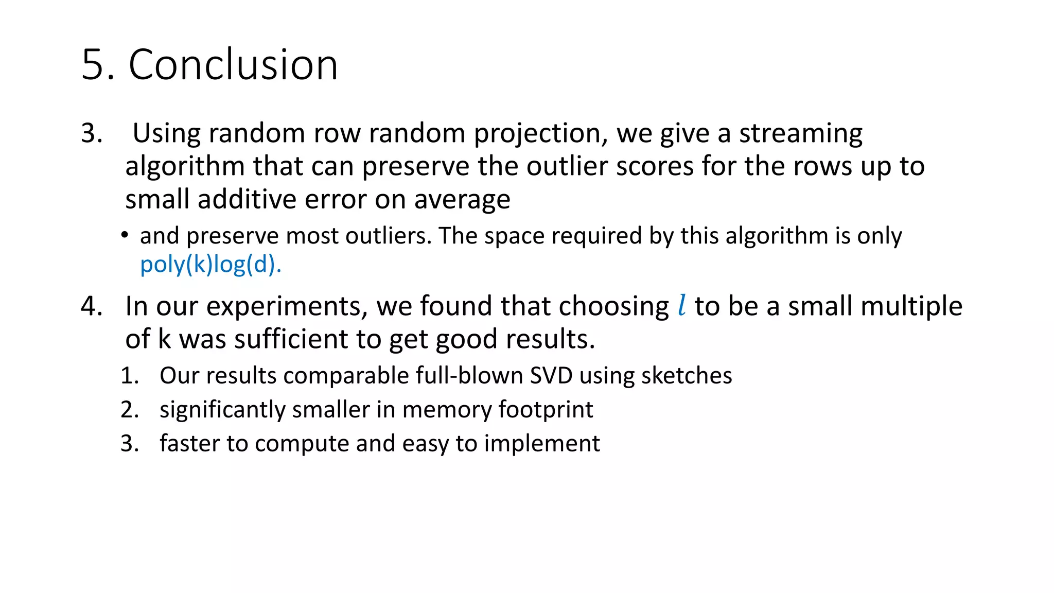
![2. Notation and Setup
• Data matrix 𝐴 ∈ 𝑅 𝑛×𝑑 s.t.
𝐴 = 𝑎 1
𝑇
; … ; 𝑎 𝑛
𝑇
𝑤ℎ𝑒𝑟𝑒 𝑎 𝑖 ∈ 𝑅 𝑑
= 𝑎(1)
, … , 𝑎(𝑑)
𝑤ℎ𝑒𝑟𝑒 𝑎
(𝑖)
∈ 𝑅 𝑛
• SVD of A: 𝐴 = 𝑈Σ𝑉 𝑇 𝑤ℎ𝑒𝑟𝑒
Σ = 𝑑𝑖𝑎𝑔 𝜎1, … , 𝜎 𝑑 , 𝜎1 ≥ ⋯ ≥ 𝜎 𝑑 > 0
𝑉 = [𝑣 1
, … , 𝑣(𝑑)
]
• Condition number of the top k subspace of A: 𝜅 𝑘 = 𝜎1
2
/𝜎 𝑘
2
• Frobenius norm: 𝐴 𝐹 = 𝑖=1
𝑛
𝑗=1
𝑑
|𝑎𝑖𝑗|2
• Operator norm: 𝐴 = 𝜎1](https://image.slidesharecdn.com/efficientanomalydetectionviamatrixsketching20190801-190802163552/75/Efficient-anomaly-detection-via-matrix-sketching-8-2048.jpg)
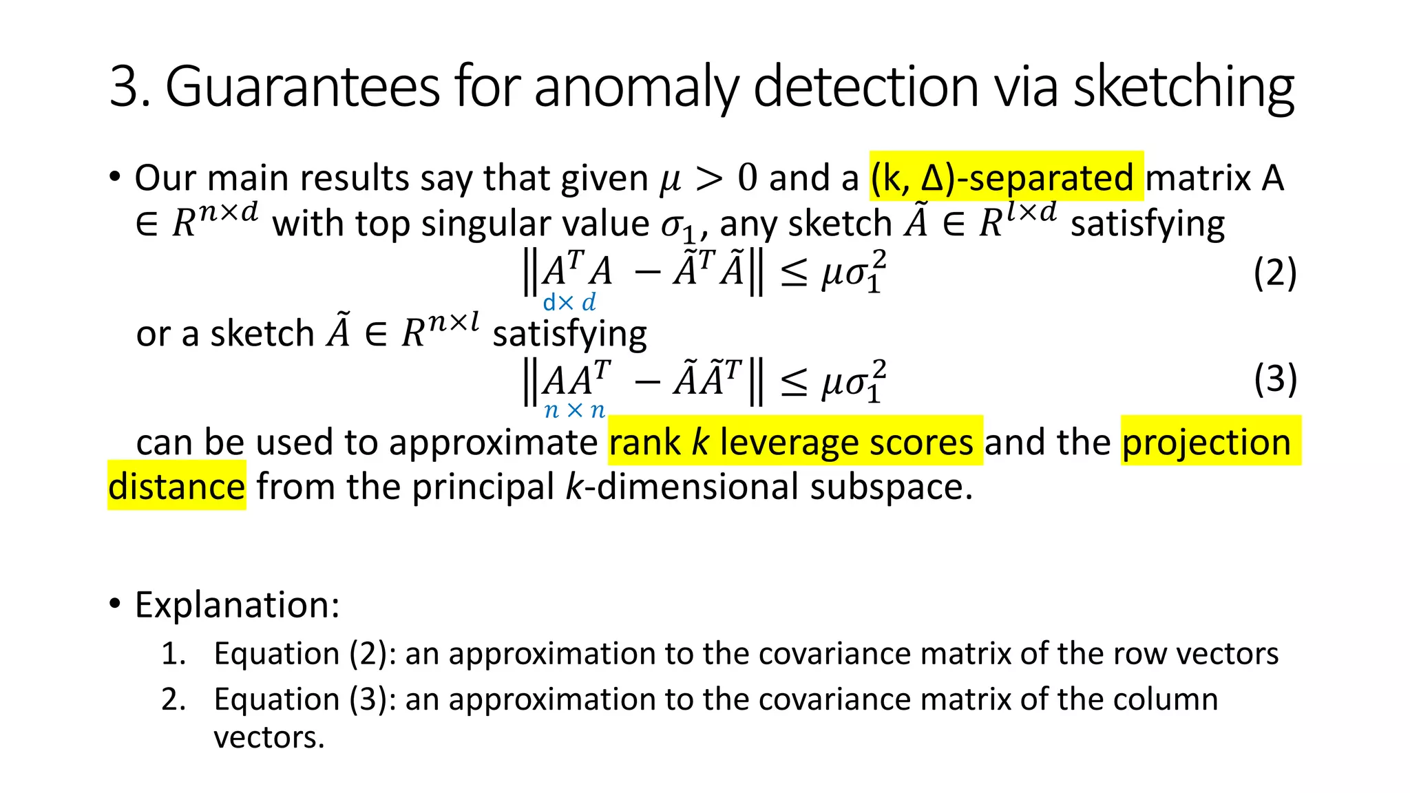
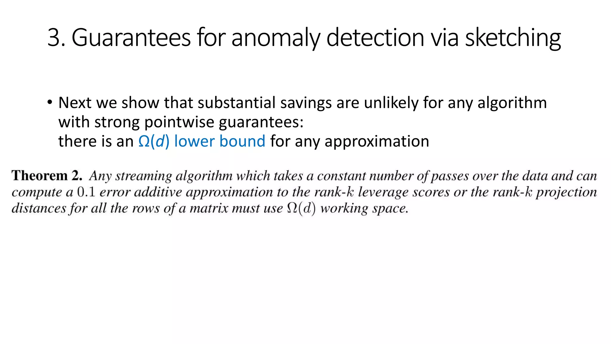
![3. Guarantees for anomaly detection via sketching
• Next, we show how to design efficient algorithms for finding
anomalies in a streaming fashion.
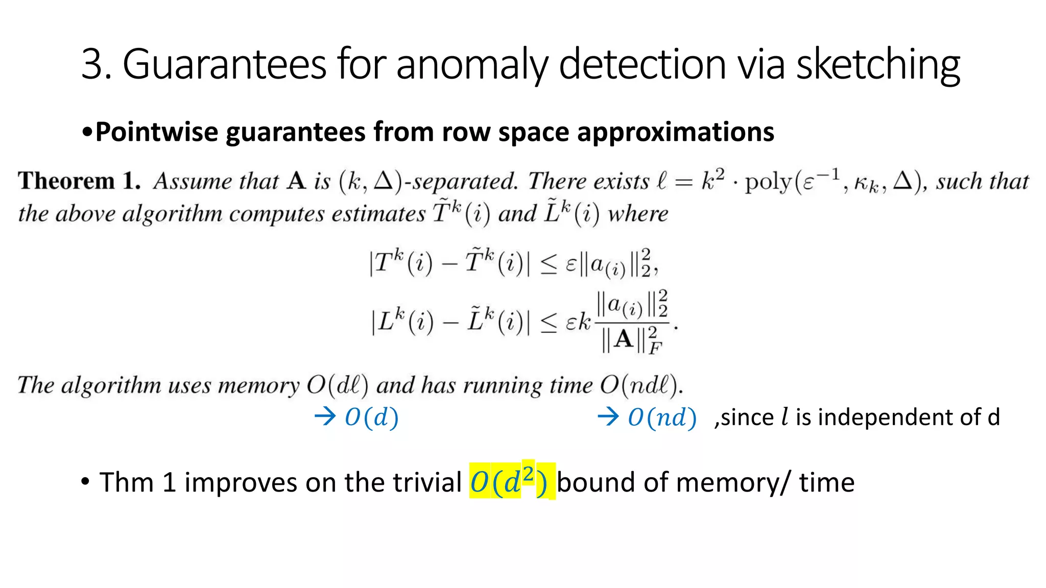
• Pointwise guarantees from row space approximations
Algorithm 1: random column projection/ row space approximation
• Sketching techs: Frequent Directions sketch [18], row-sampling [19], random
column projection, …
(𝑛 → 𝑙)](https://image.slidesharecdn.com/efficientanomalydetectionviamatrixsketching20190801-190802163552/75/Efficient-anomaly-detection-via-matrix-sketching-13-2048.jpg)
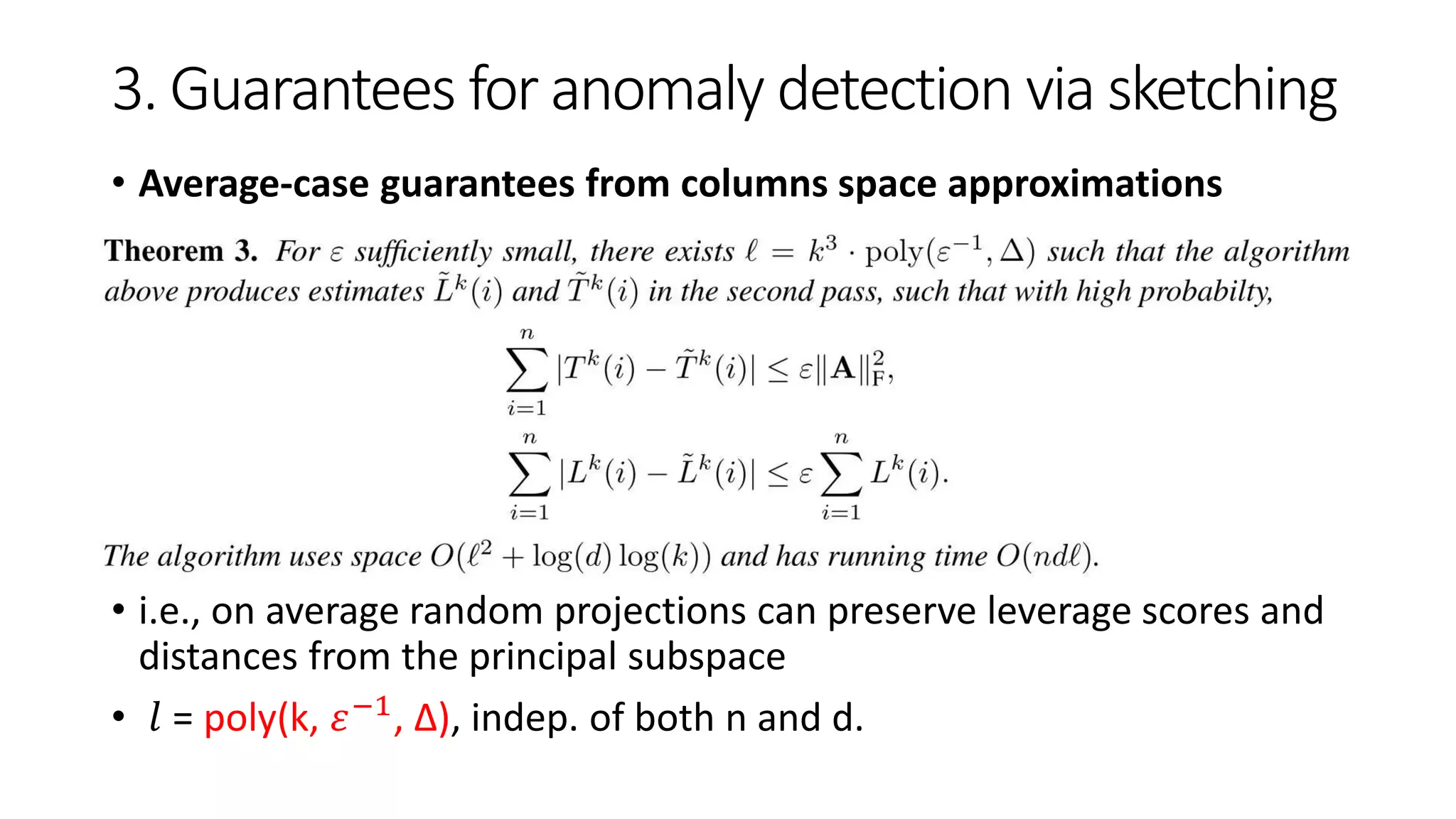
![3. Guarantees for anomaly detection via sketching
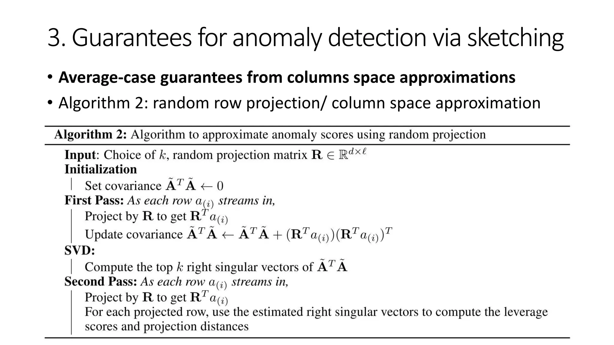
• Average-case guarantees from columns space approximations
Even though the sketch gives column space approximations (i.e.
𝐴𝐴 𝑇 approximation satisfying Equ. (3))
Our goal is still to compute the row anomaly scores from 𝐴 𝑇 𝐴
• E.g., by random matrix 𝑹 ∈ 𝑹 𝑑×𝑙 s.t. 𝑟𝑖𝑗 ~
𝑖.𝑖.𝑑 𝑈{±1}) where 𝑙 = 𝑂(𝑘/𝜇2) [27]
sketch 𝑨 = 𝑨𝑹 for which returns the anomaly scores
Space consumption
• For 𝐴 𝑇
𝐴 𝑂 𝑙2
• For 𝑹 able to be pseudorandom [28-30] 𝑂 log(𝑑)](https://image.slidesharecdn.com/efficientanomalydetectionviamatrixsketching20190801-190802163552/75/Efficient-anomaly-detection-via-matrix-sketching-16-2048.jpg)
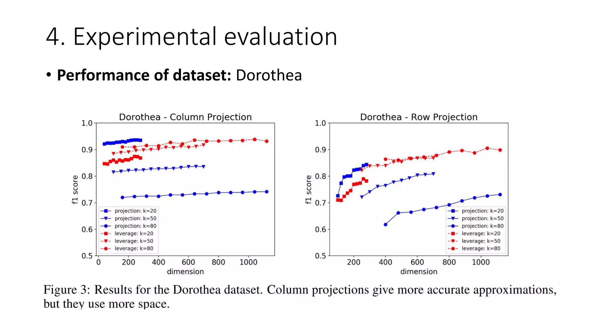
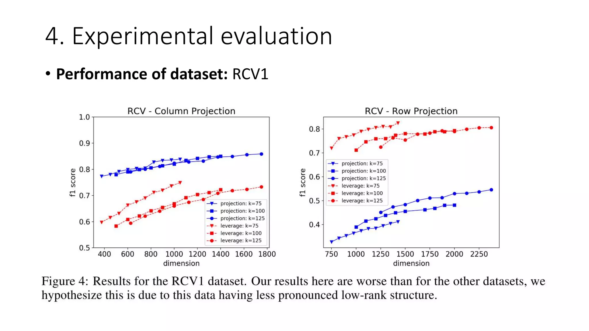
![4. Experimental evaluation
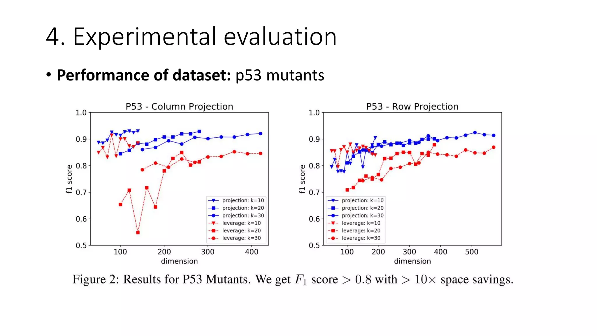
• Data: (1) p53 mutants [32], (2) Dorothea [33], (3) RCV1 [34]
All available from the UCI Machine Learning Repository,
• Ground truth: to decide anomalies
• We compute the rand k anomaly scores using a full SVD, and then label the η
fraction of points with the highest anomaly scores to be outliers.
1. k chosen by examining the explained variance of the datatset: typically between (10, 125)
2. η chosen by examining the histogram of the anomaly score; typically between (0.01, 0.1)](https://image.slidesharecdn.com/efficientanomalydetectionviamatrixsketching20190801-190802163552/75/Efficient-anomaly-detection-via-matrix-sketching-20-2048.jpg)


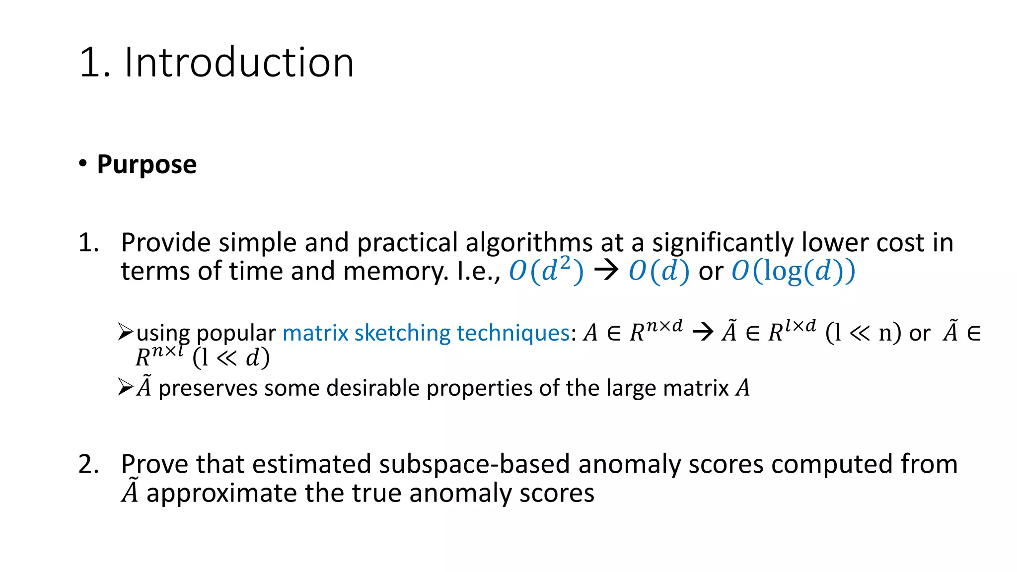
The document discusses efficient anomaly detection in high-dimensional streaming data using matrix sketching techniques. It outlines the limitations of standard PCA-based approaches due to high computational costs and presents algorithms that approximate anomaly scores using significantly less memory and time. Experimental evaluations demonstrate that the proposed algorithms can achieve comparable results to full SVD with a reduced computational footprint.


![[DSC Europe 25] Jovan Bogicevic - Legacy to AI-Driven Defense: Transforming D...](https://cdn.slidesharecdn.com/ss_thumbnails/rsarluadt563hntyfc8q-3-251211083849-3e7bc4c0-thumbnail.jpg?width=640&height=640&fit=bounds)


![[DSC Europe 25] Danica Soc - The Science Behind Marketing: Experimentation me...](https://cdn.slidesharecdn.com/ss_thumbnails/c0nofsggs9gw5ucmallr-3-251216103155-56bd64d1-thumbnail.jpg?width=640&height=640&fit=bounds)
![[DSC Europe 25] Bassam Maharmeh - Artificial Intelligence: Opportunities and ...](https://cdn.slidesharecdn.com/ss_thumbnails/thhfmr2fqpawzj7hsjpg-5-251211083048-2c23204f-thumbnail.jpg?width=640&height=640&fit=bounds)


![[DSC Europe 25] Dusan Nesic - Securing Tomorrow’s Infrastructure: Why Cyber-P...](https://cdn.slidesharecdn.com/ss_thumbnails/qikbszfftyowjm2q6duw-1-251211083848-8f2ead6b-thumbnail.jpg?width=640&height=640&fit=bounds)
![[DSC Europe 25] Katherine Forrest - AI NOW: Understanding the Velocity of Cha...](https://cdn.slidesharecdn.com/ss_thumbnails/wvvbruqfrci0sfq9xwgb-4-251212104007-e5ad1987-thumbnail.jpg?width=640&height=640&fit=bounds)

![[DSC Europe 25] Uros Pesic - The Reality of AI in Marketing.pdf](https://cdn.slidesharecdn.com/ss_thumbnails/rtkodnmtycovsllvzsyn-9-251215095918-b0c6bfe3-thumbnail.jpg?width=640&height=640&fit=bounds)
![[DSC Europe 25] Hans Kleinsman - The Compliance Gearbox: How Tax Tech Mediate...](https://cdn.slidesharecdn.com/ss_thumbnails/dxdytie1toel0hr90bjs-2-251212103250-174fdbe7-thumbnail.jpg?width=640&height=640&fit=bounds)
![[DSC Europe 25] Nikolay Burlutskiy - Best Practices for Building Enterprise M...](https://cdn.slidesharecdn.com/ss_thumbnails/uirvaiuvq8y1w8hzd9tx-7-251212103249-2619edb4-thumbnail.jpg?width=640&height=640&fit=bounds)