Downloaded 68 times


This document provides an overview of stochastic processes and Markov chains. It defines stochastic processes as families of random variables indexed by time. Markov chains are a type of stochastic process where the future state depends only on the present state, not on the past. The document discusses examples of Markov chains, transition matrices, classification of states as transient or persistent, and properties like irreducibility. It aims to introduce key concepts in stochastic processes and Markov chains.
Md. Menhazul Abedin introduces himself and the topic of Statistics III, focusing on Stochastic Processes and Markov Chains.
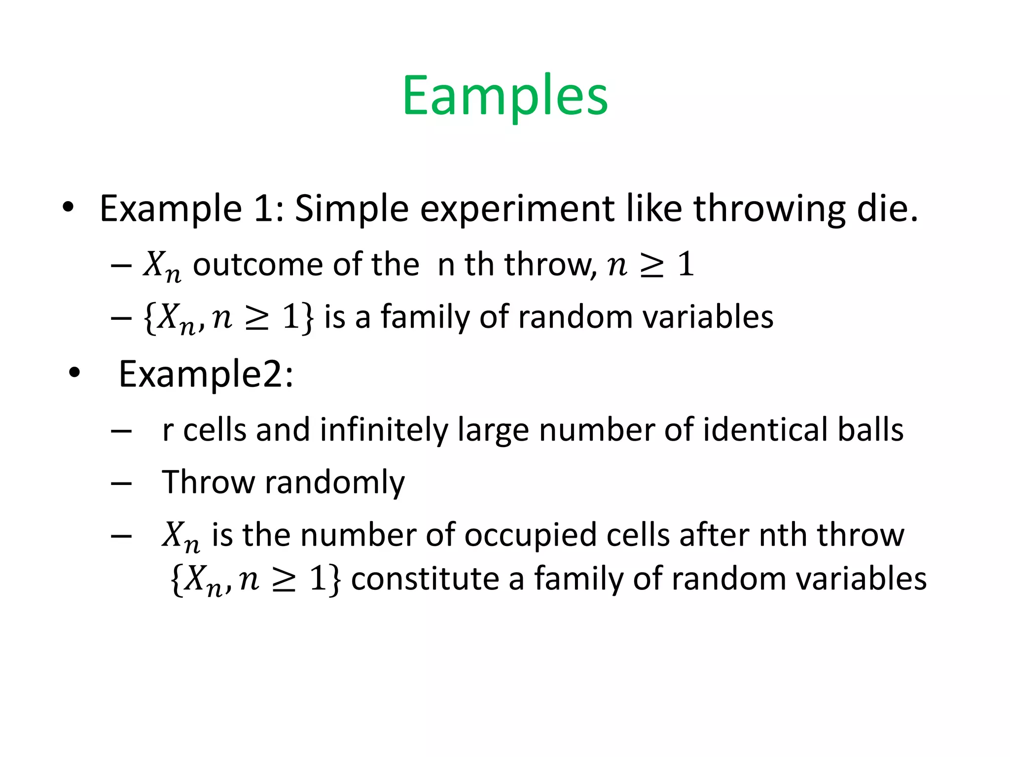
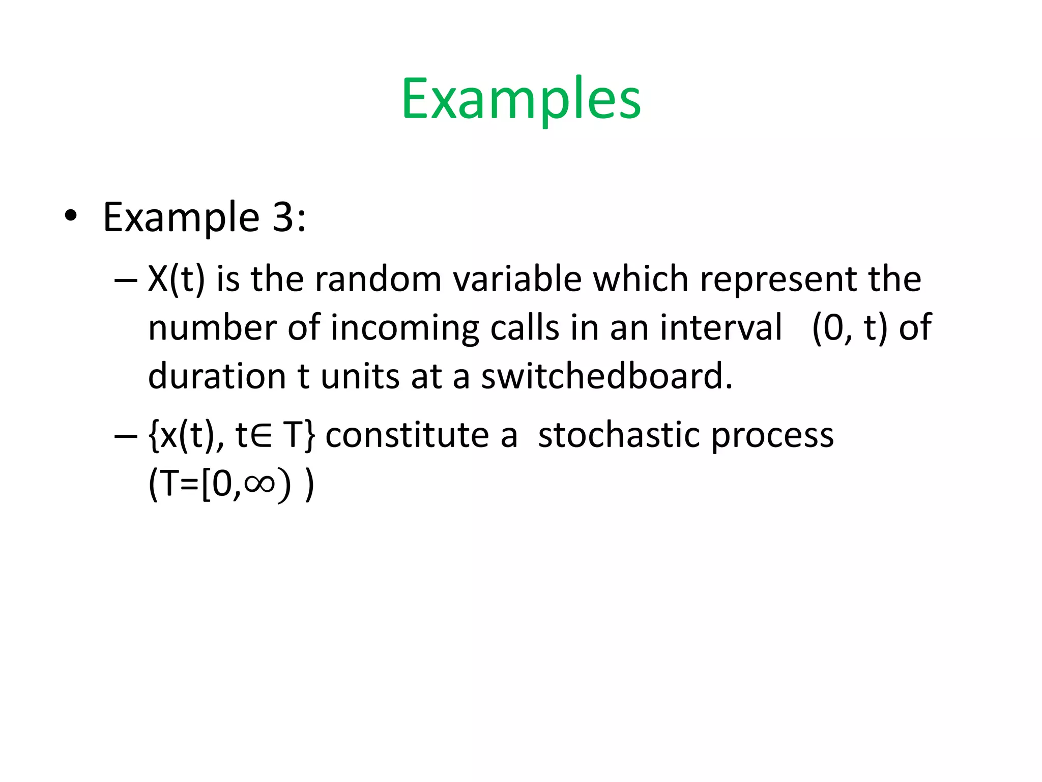
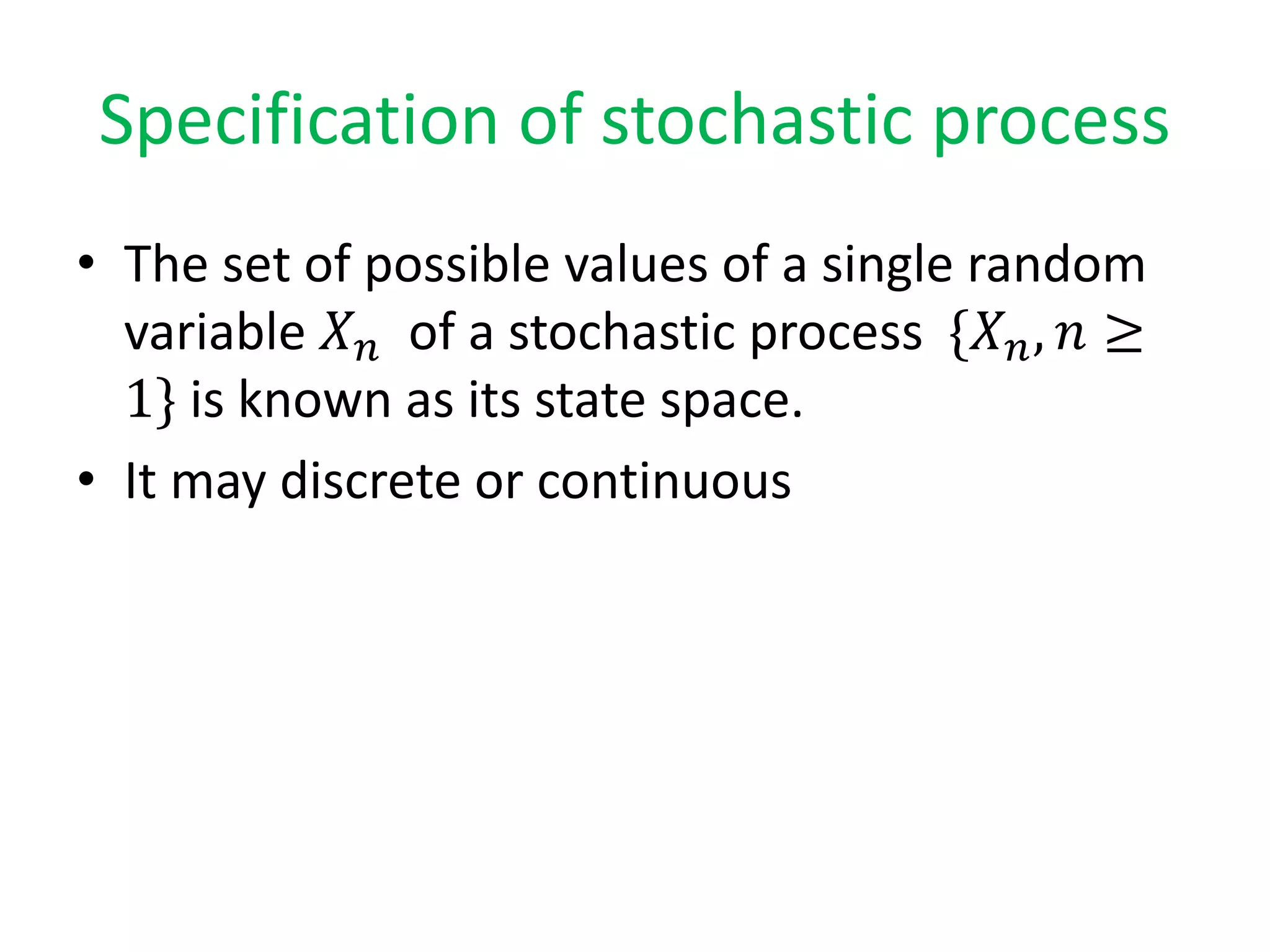
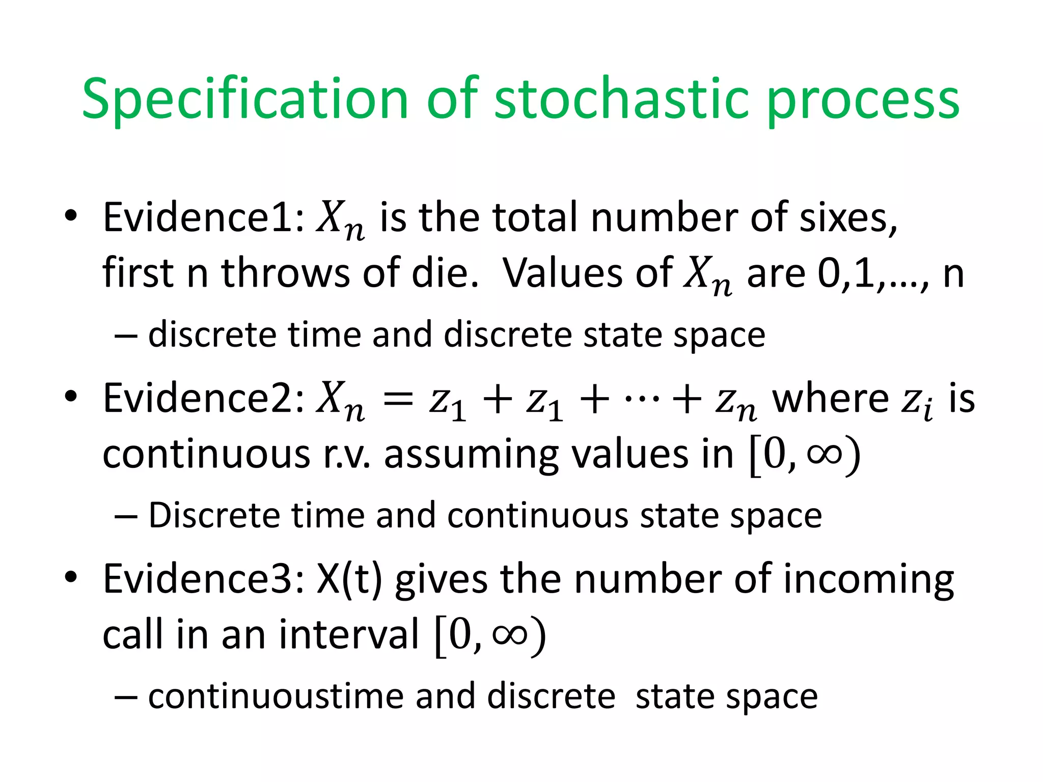
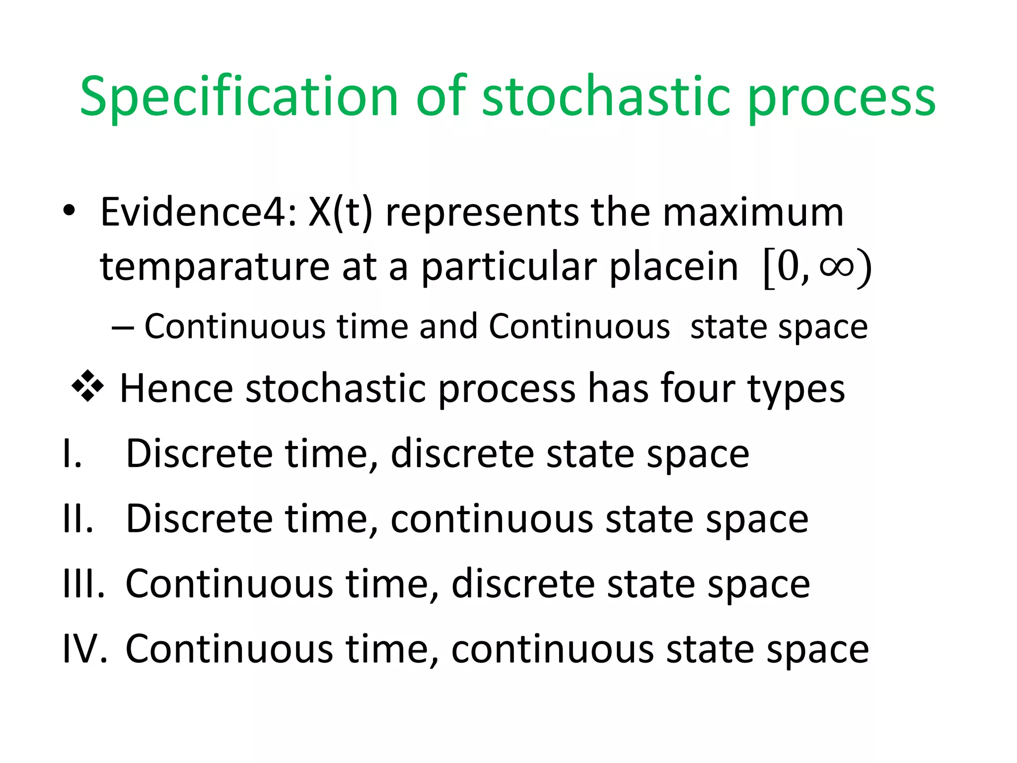
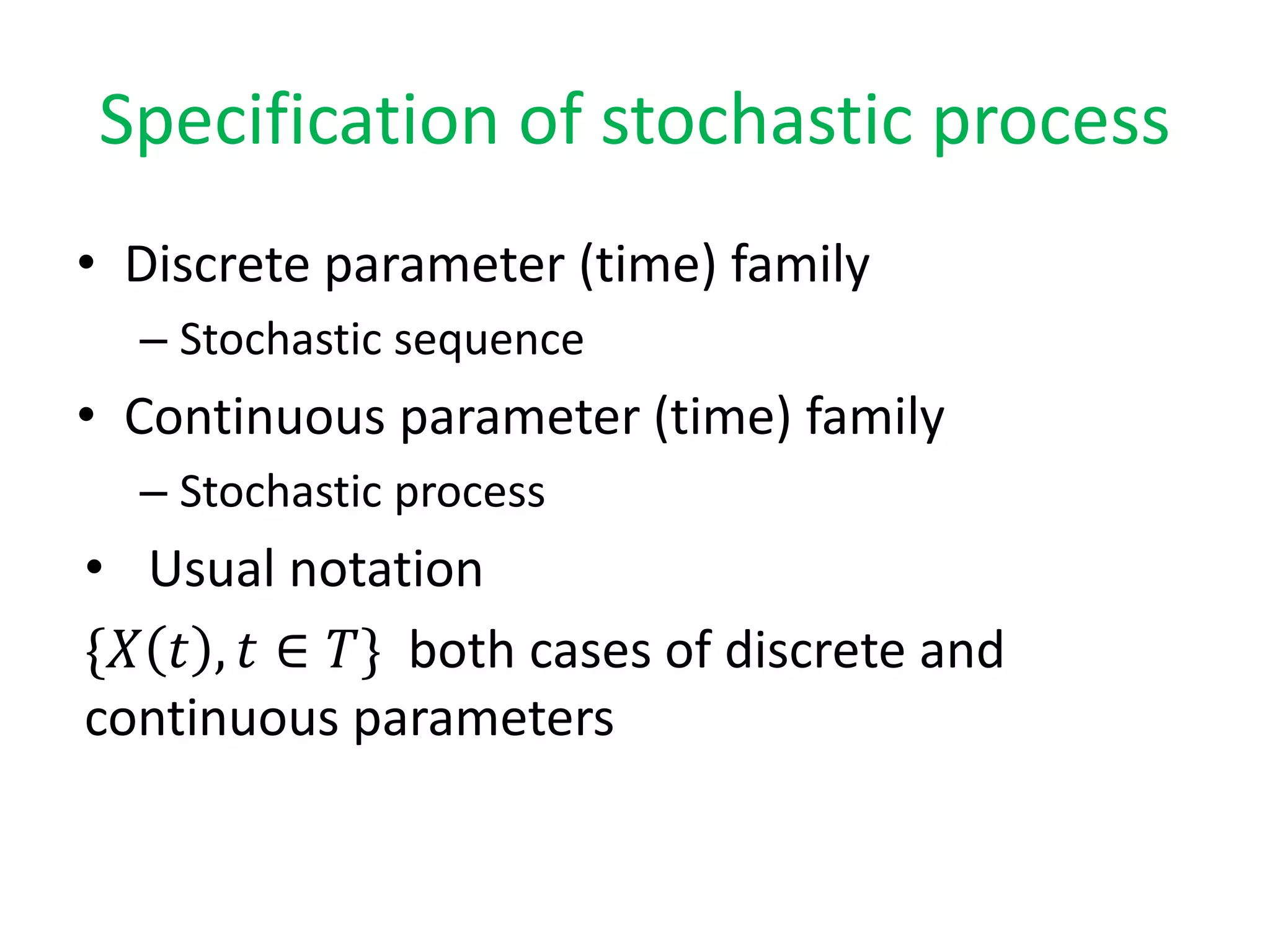
Stochastic Processes are discussed as realistic probability models that change over time, with applications in various fields and concepts like state space. Various examples illustrate stochastic processes, including random variables related to die throws and incoming calls.
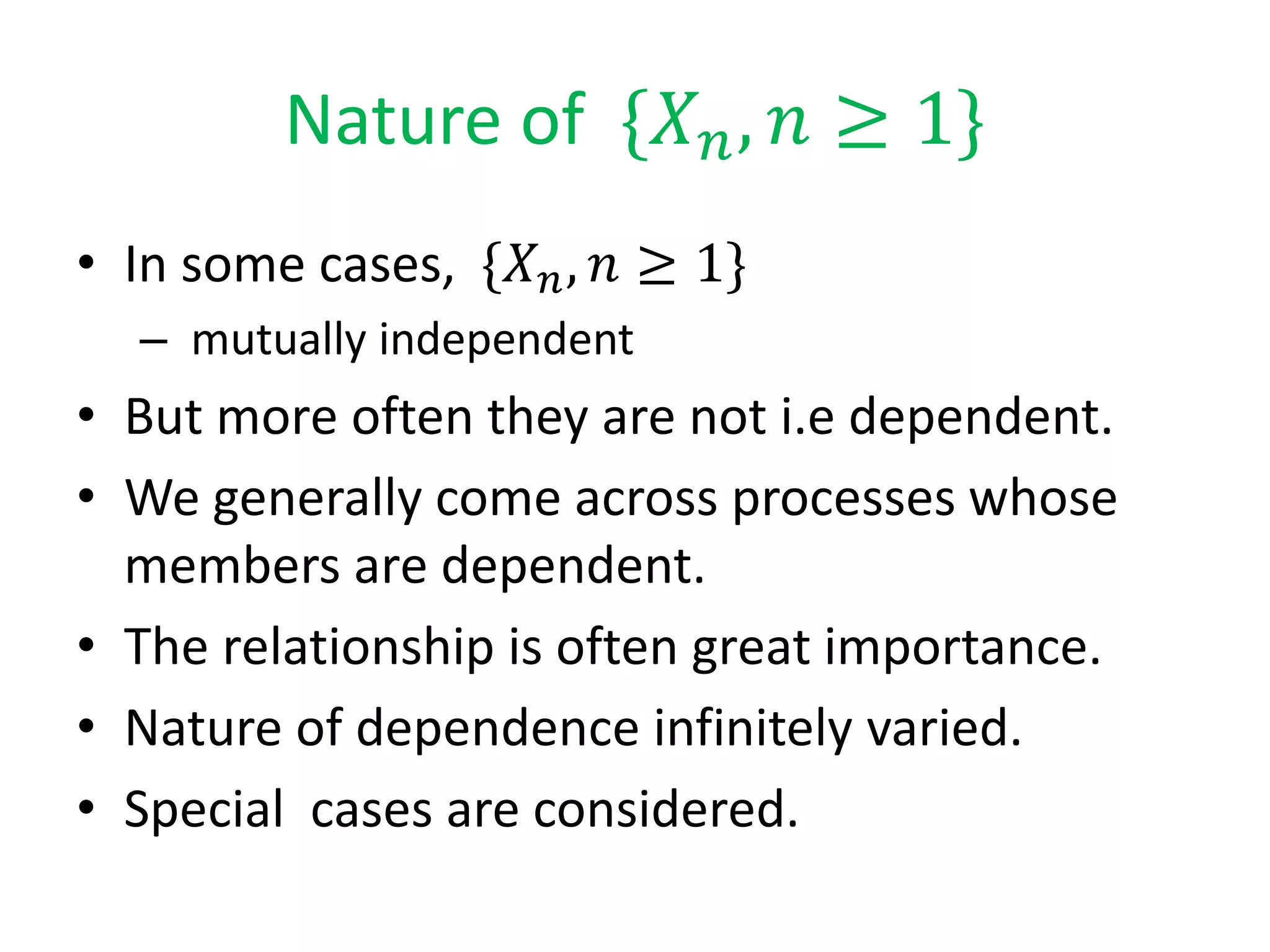
Discusses dependencies in random variables of stochastic processes, highlighting the importance of relationships.
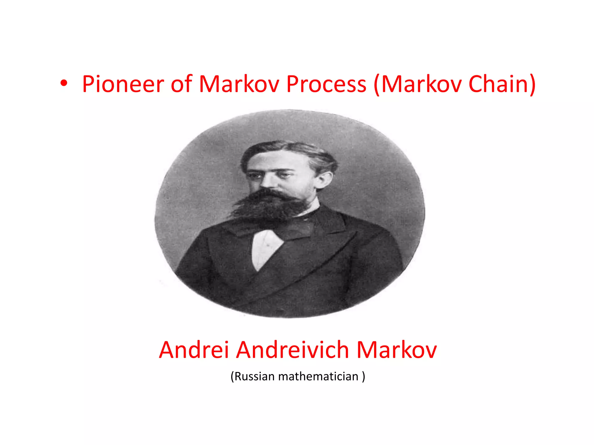
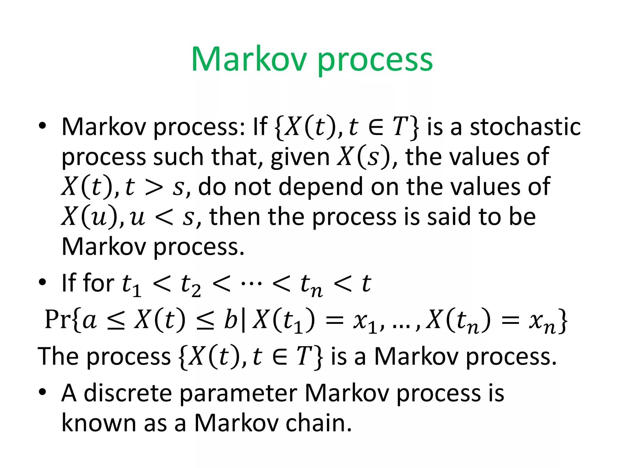
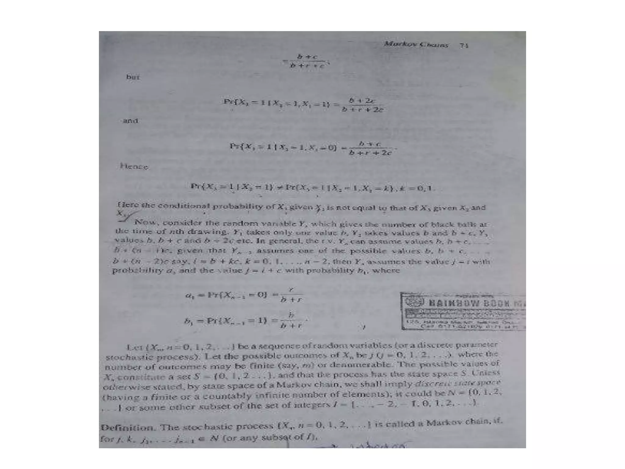
Introduction to Markov processes, including definitions and key figures like Andrei Andreivich Markov.
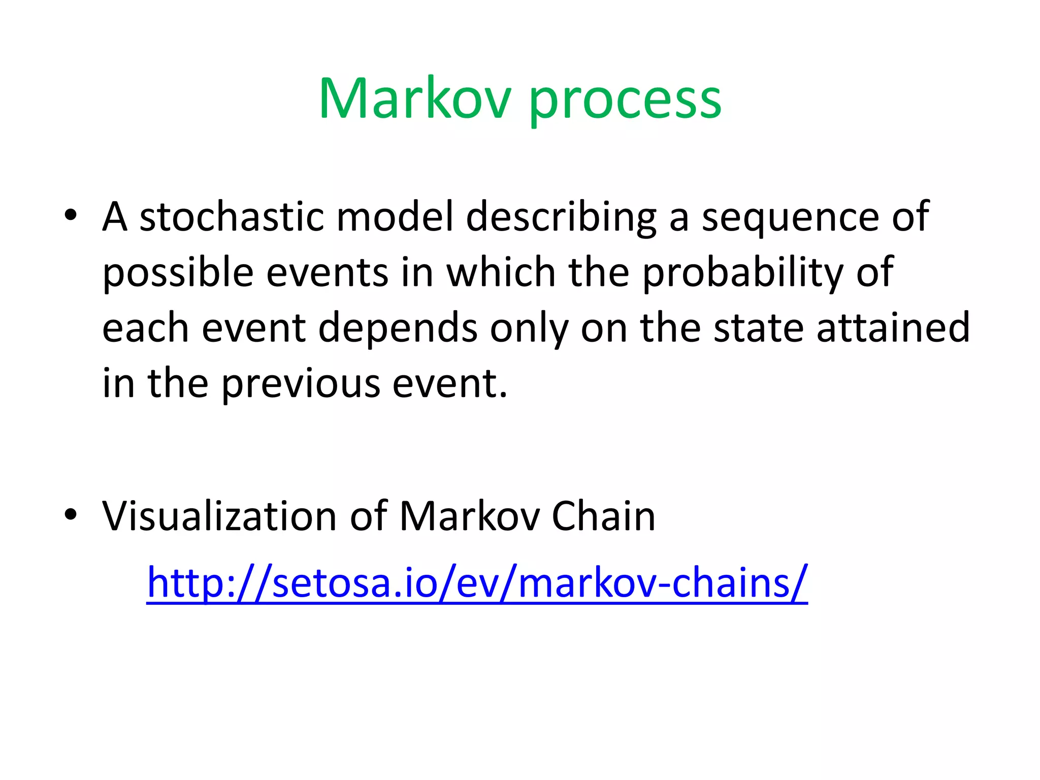
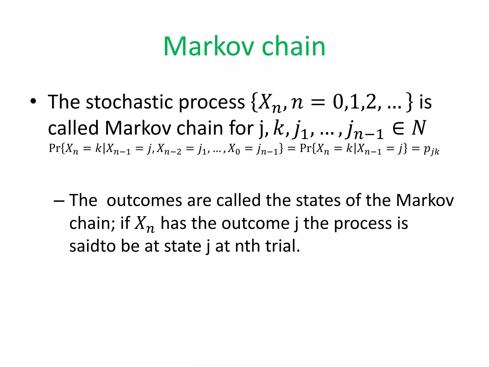
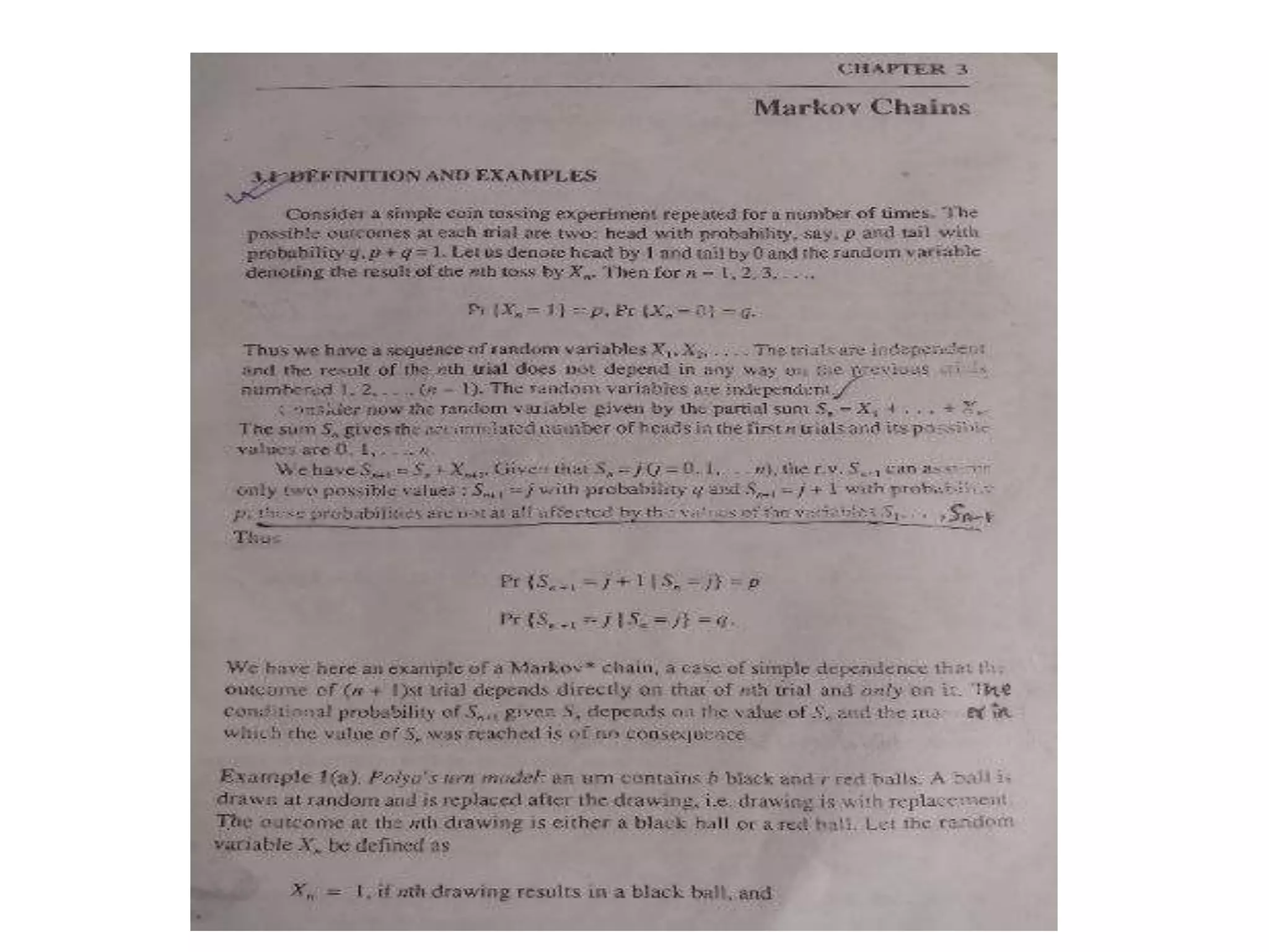
Describes Markov chains, their stochastic nature, and how the probability of events depends on previous states.
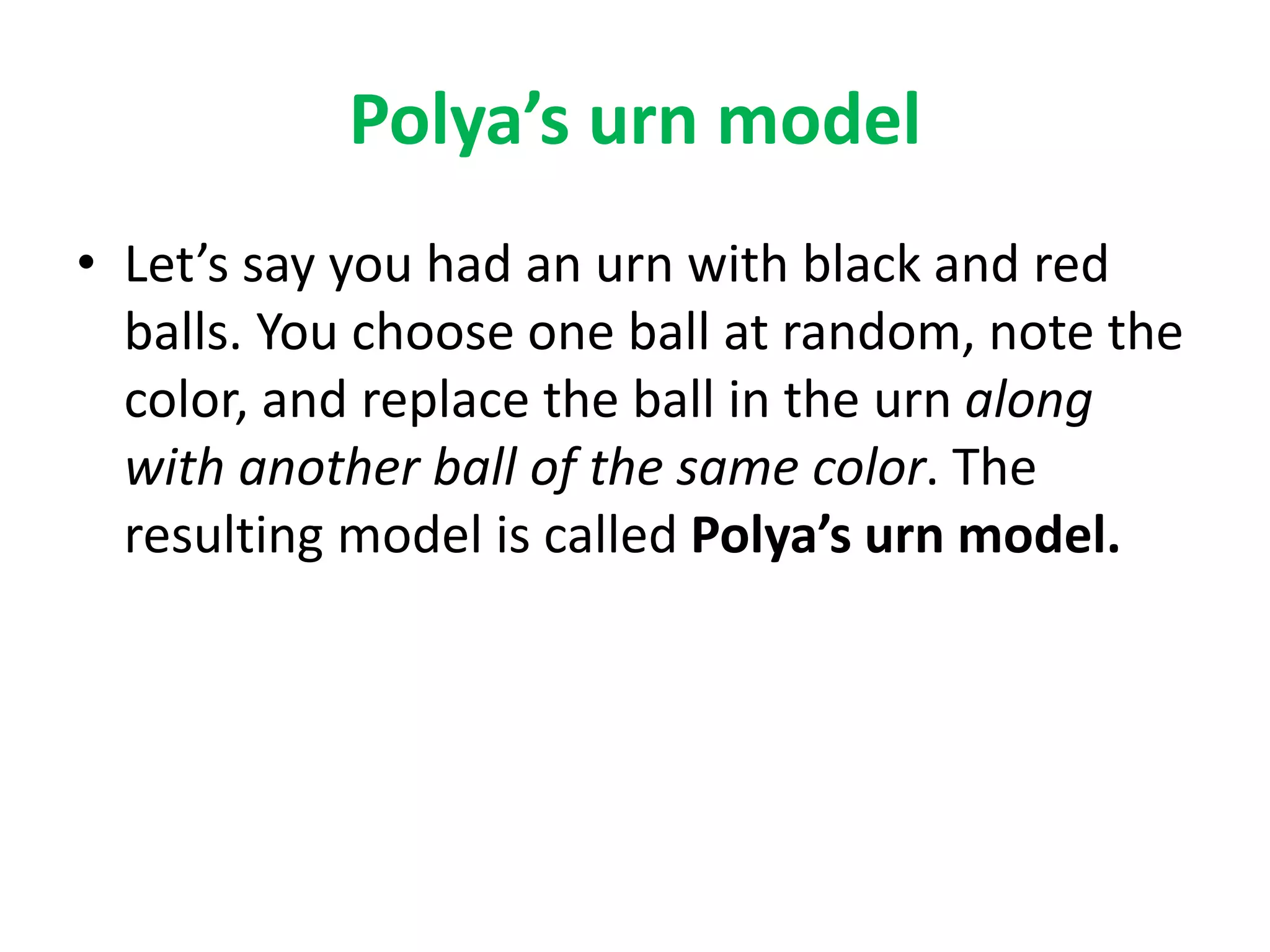
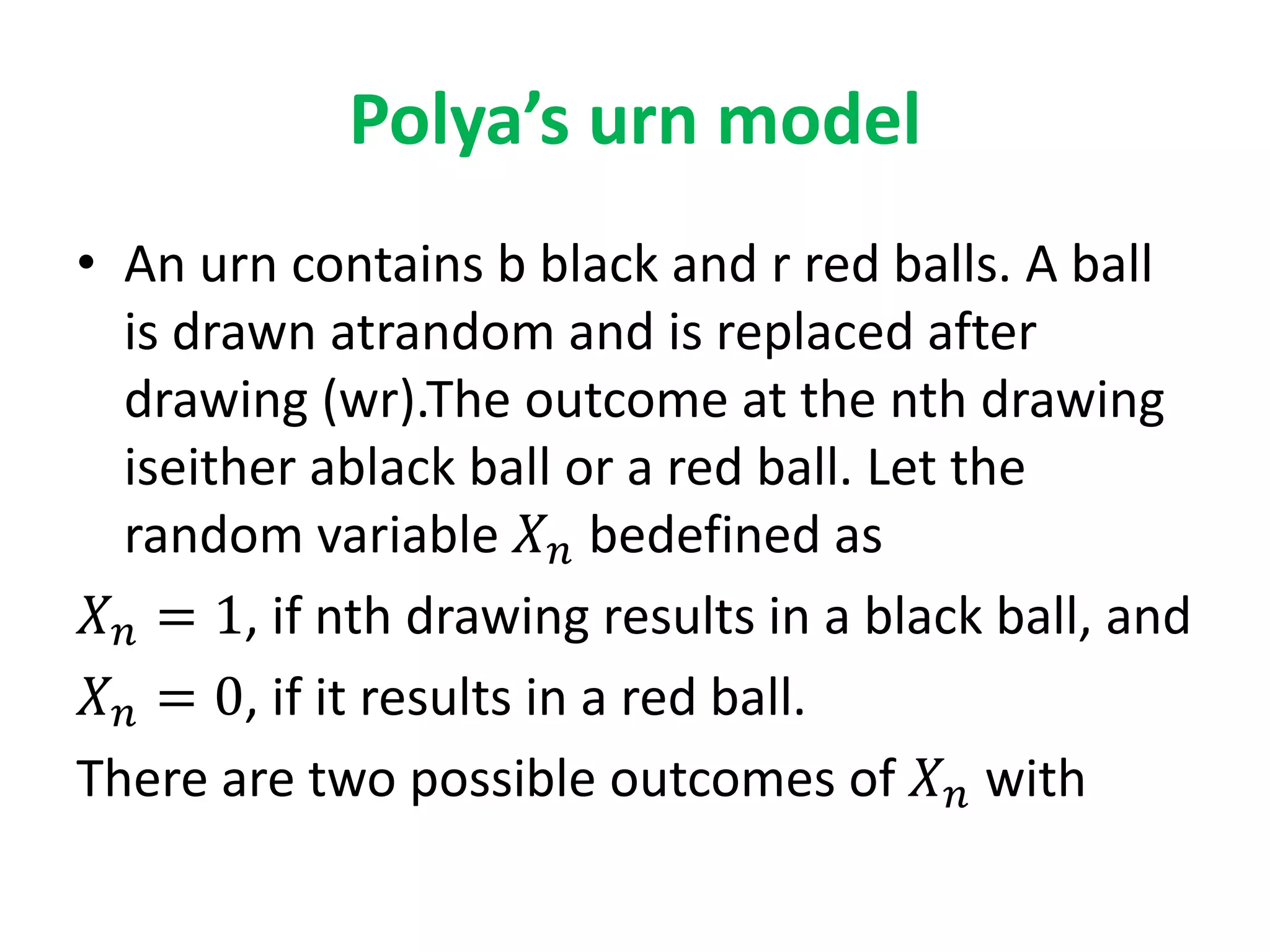
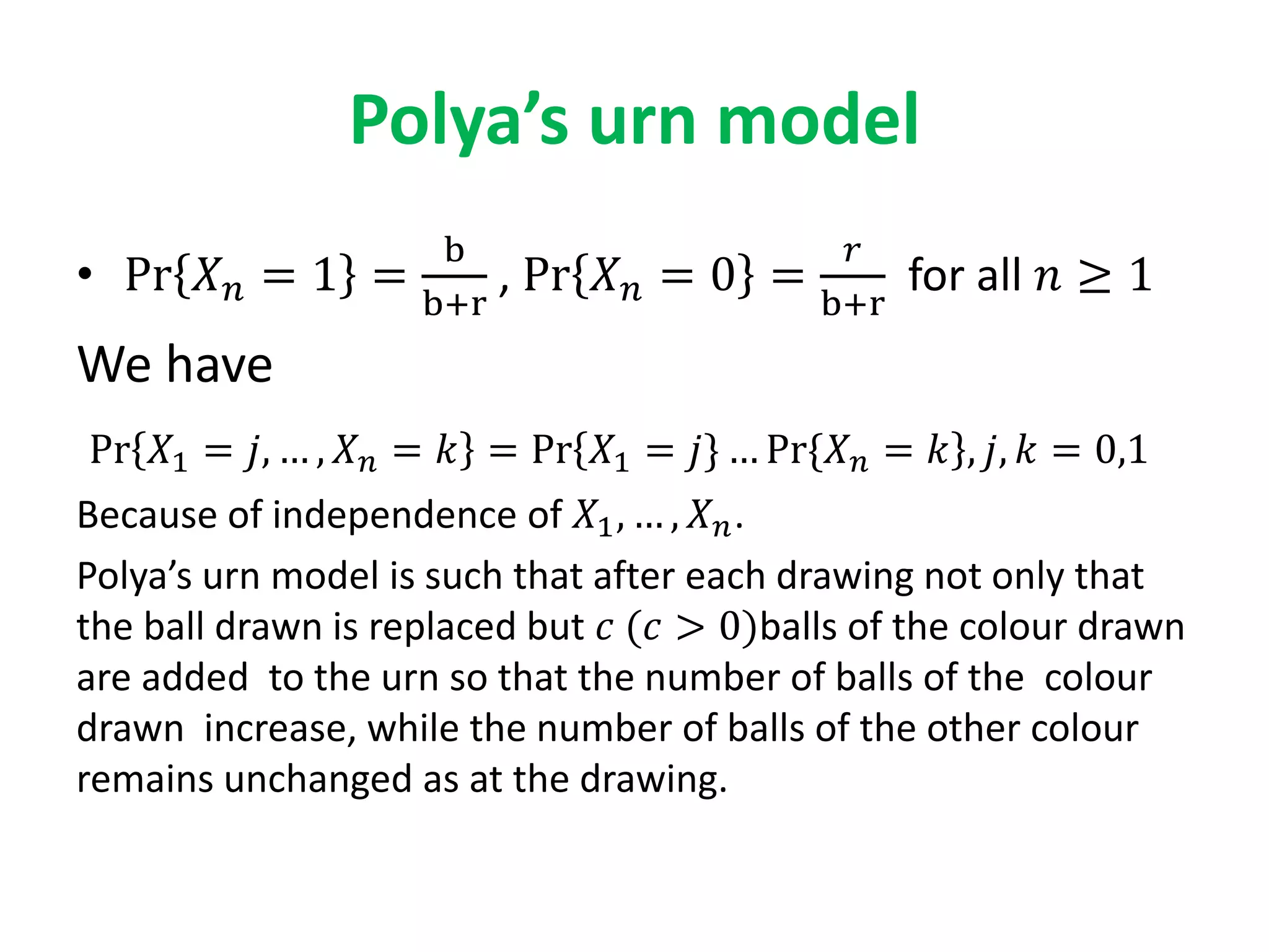
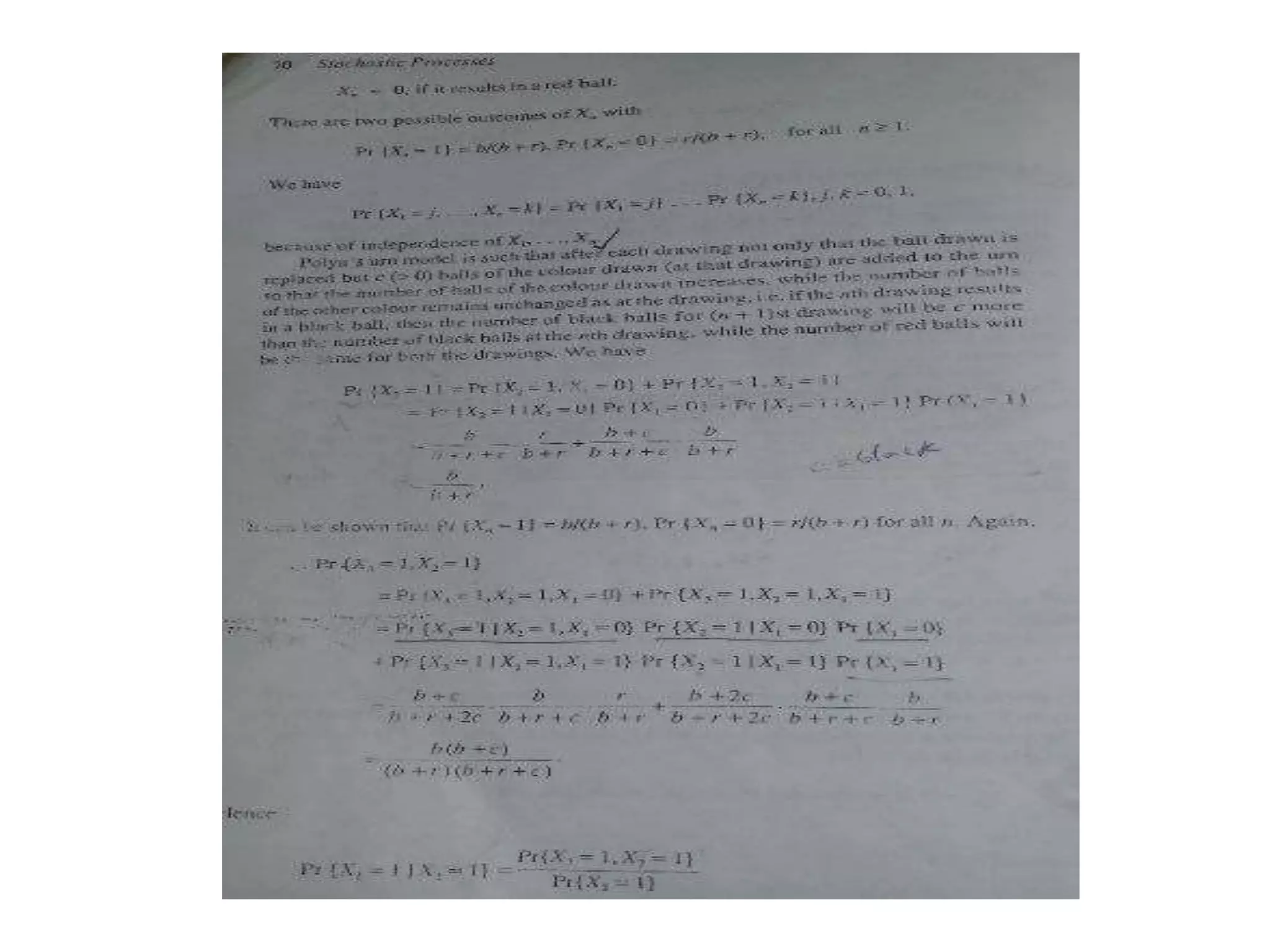
Polya's urn model is explained with examples of color selection, showcasing random variable outcomes.
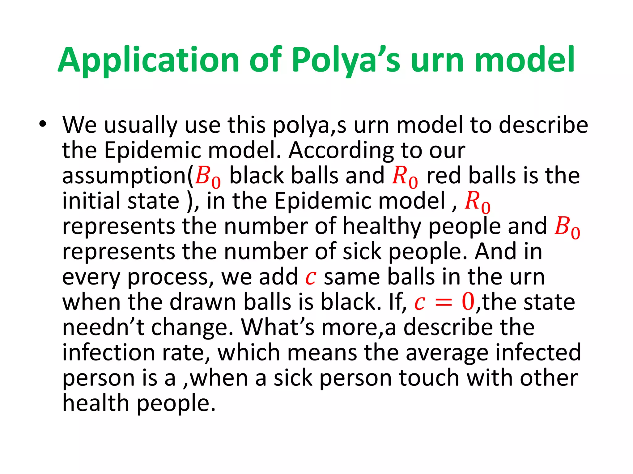
Discusses the application of Polya's urn model to epidemic modeling, with initial states representing healthy and sick individuals.
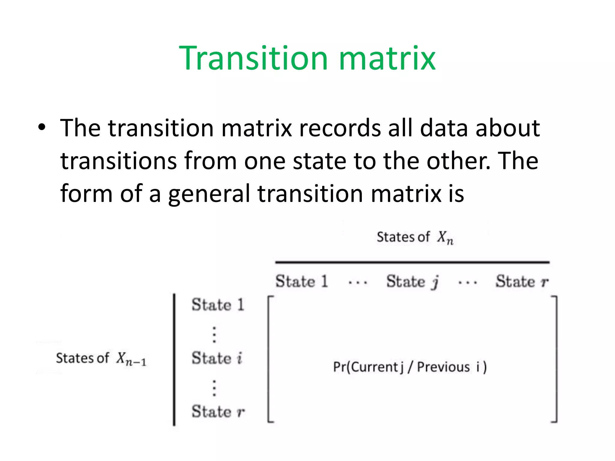
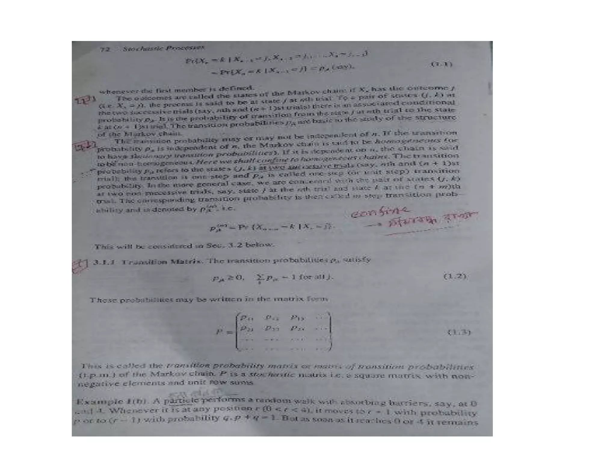
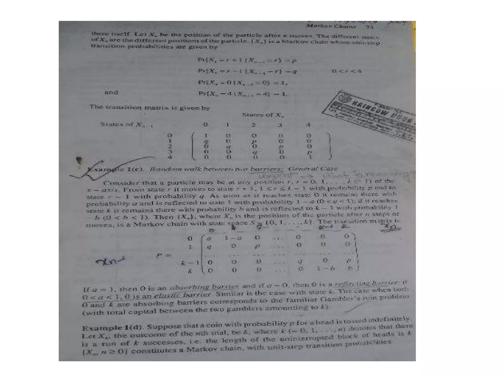
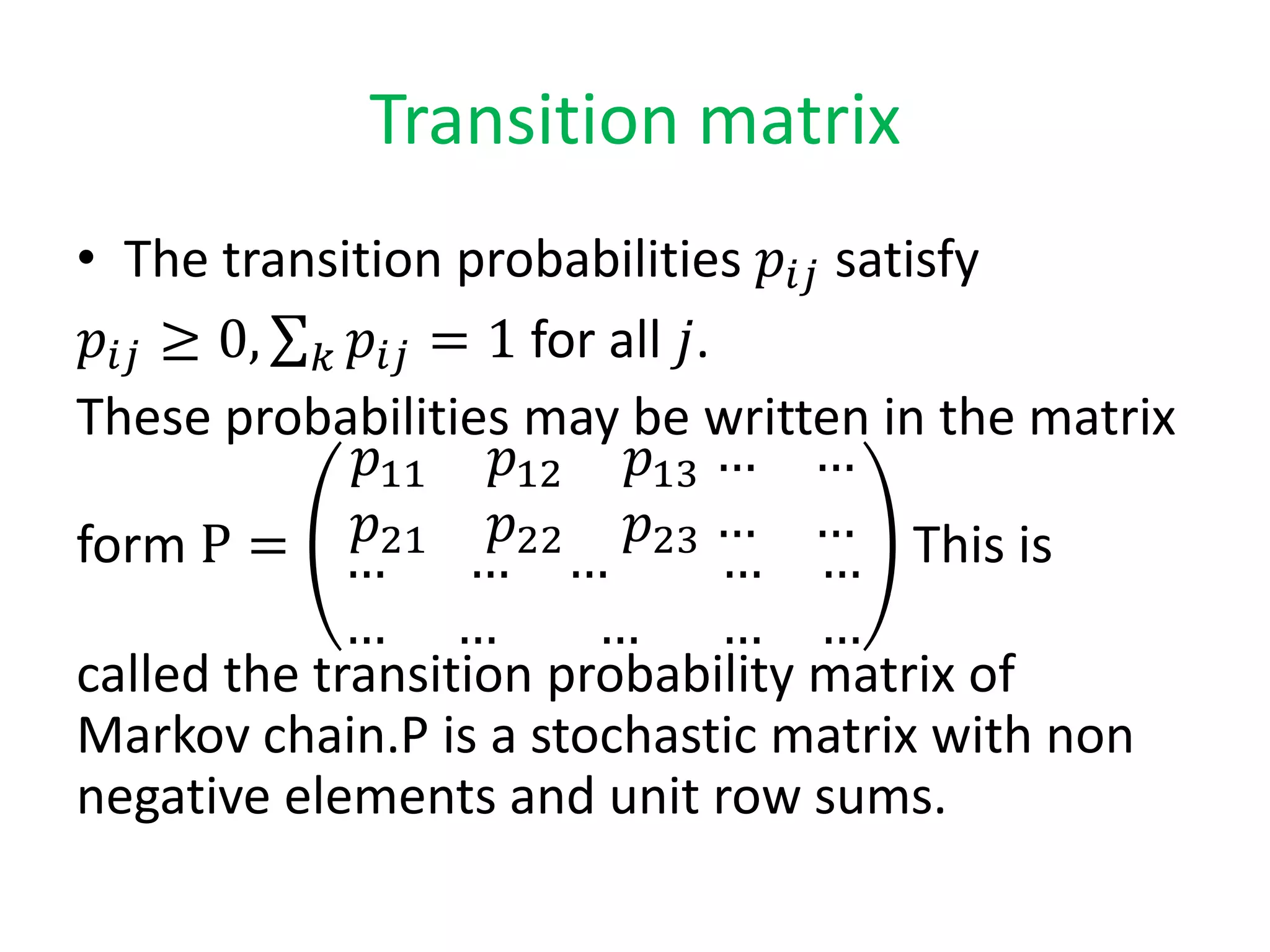
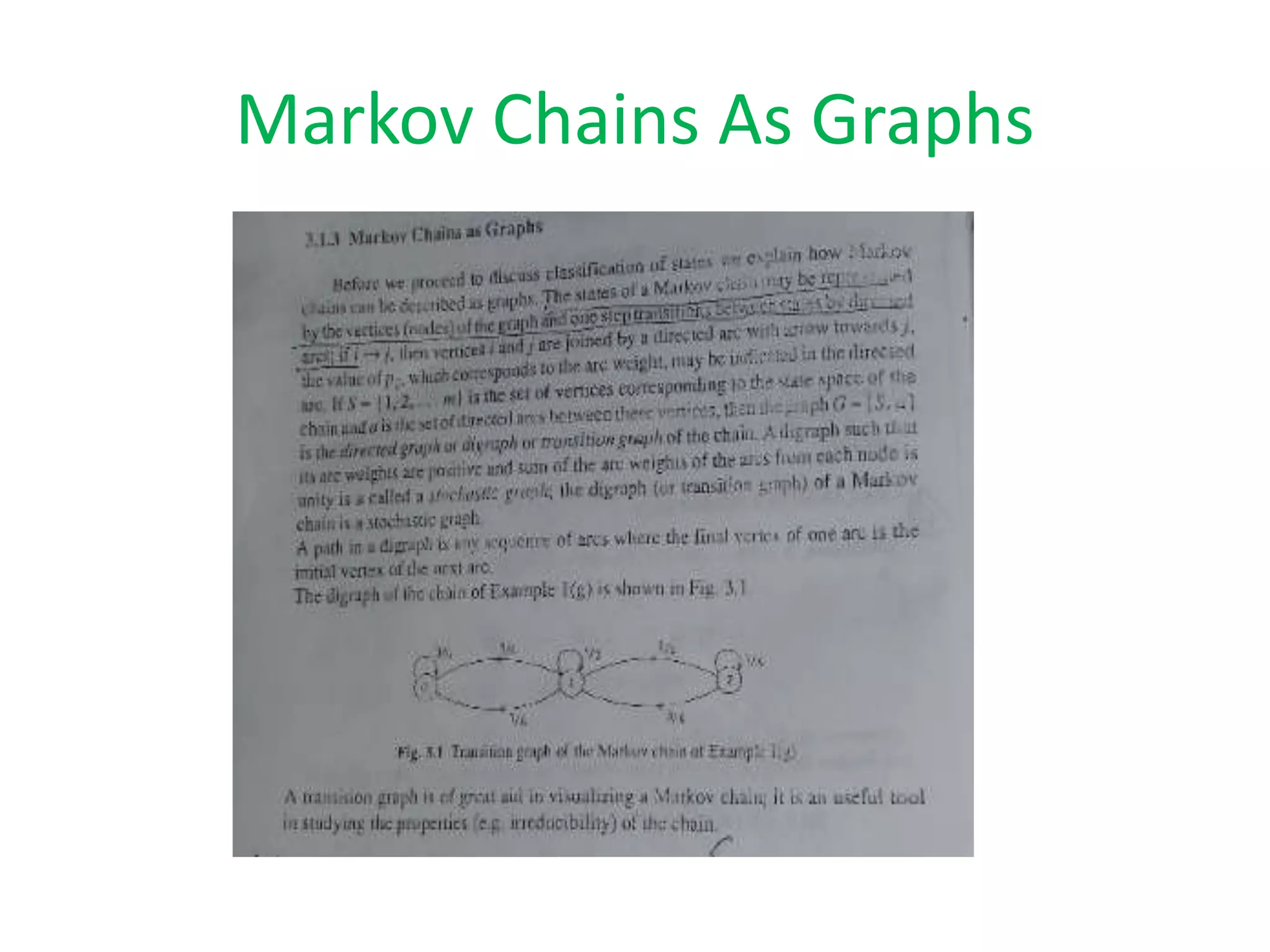
Introduction to the Transition Matrix in Markov chains, detailing its properties and structure.
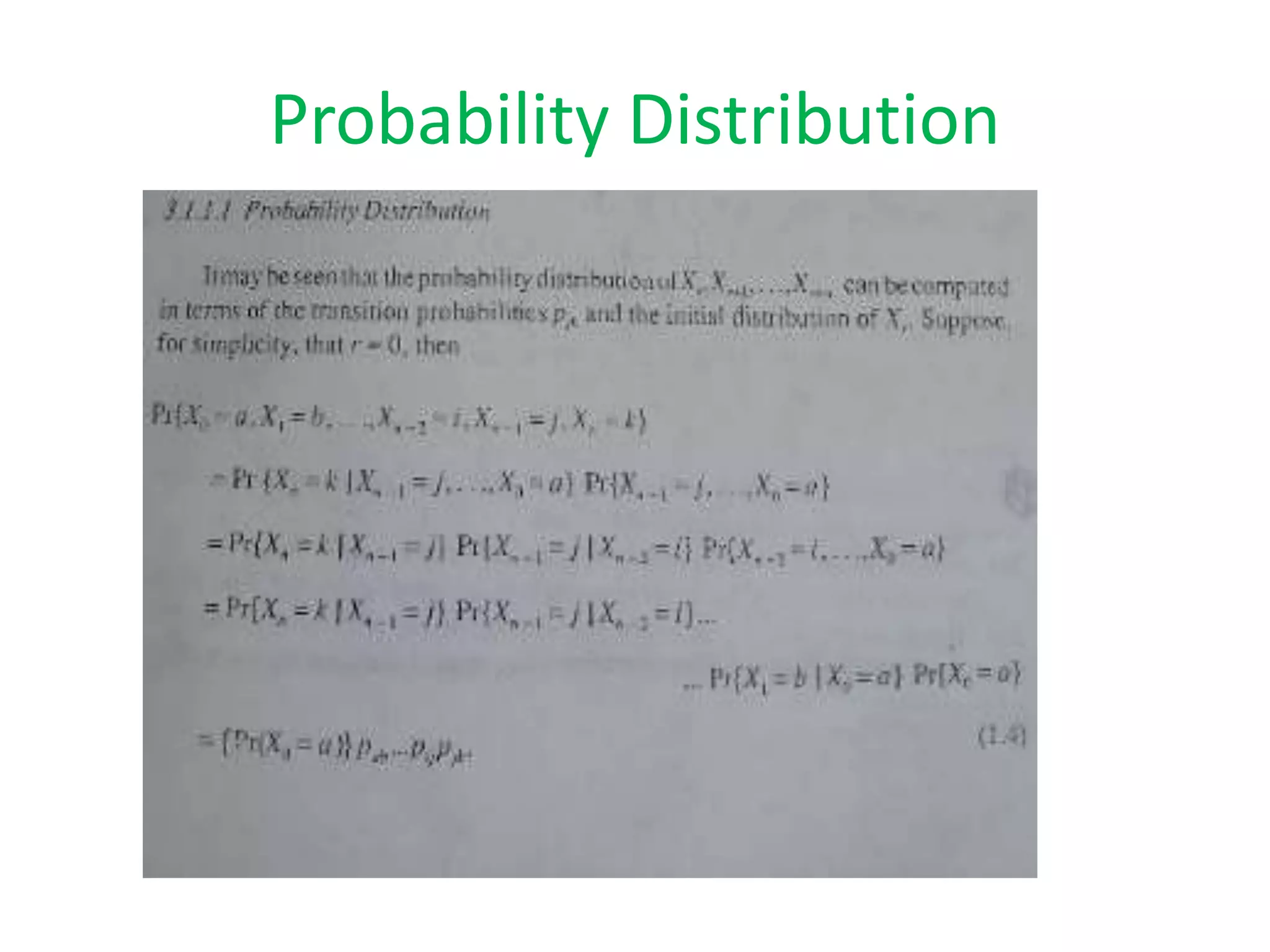
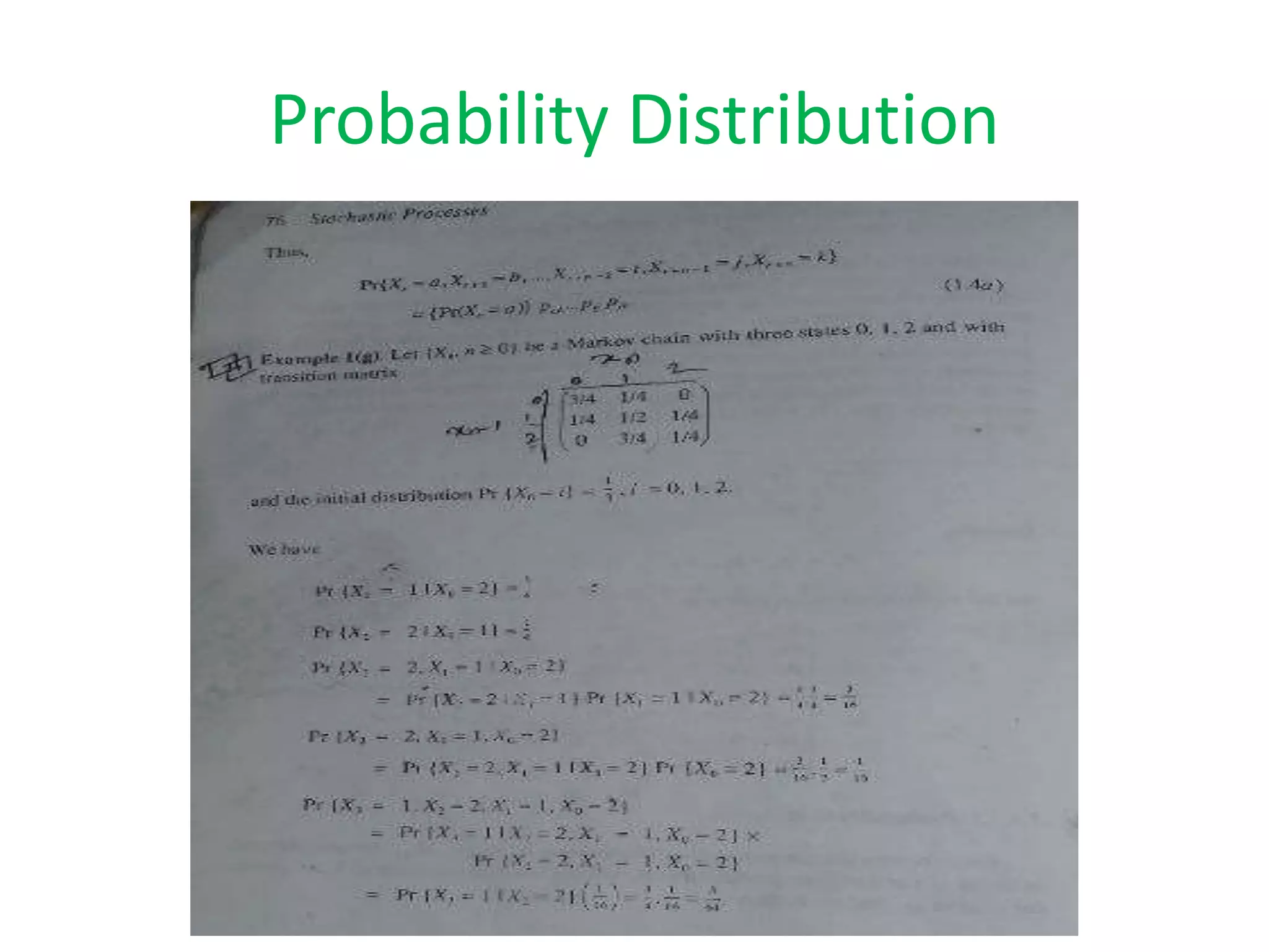
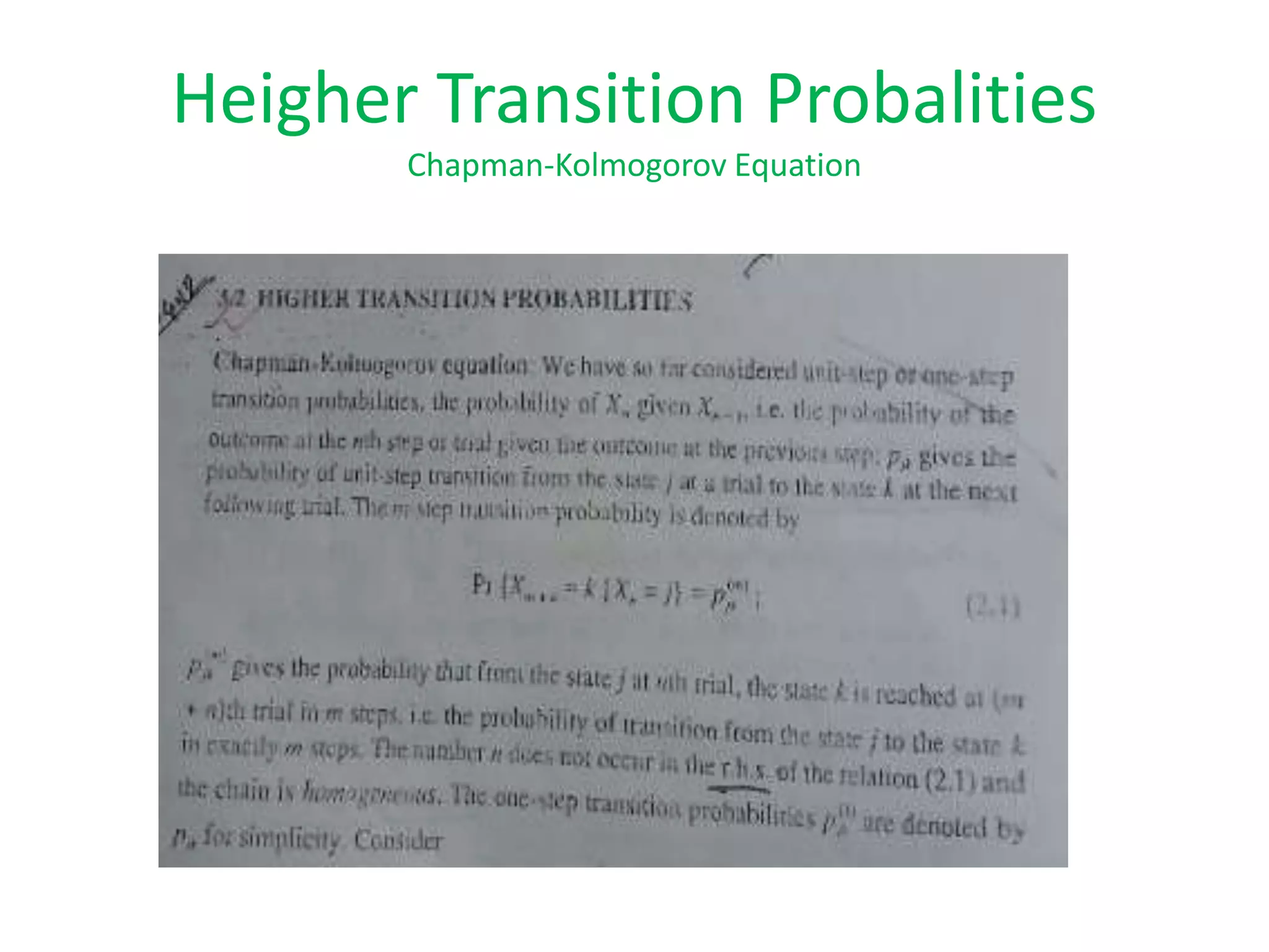
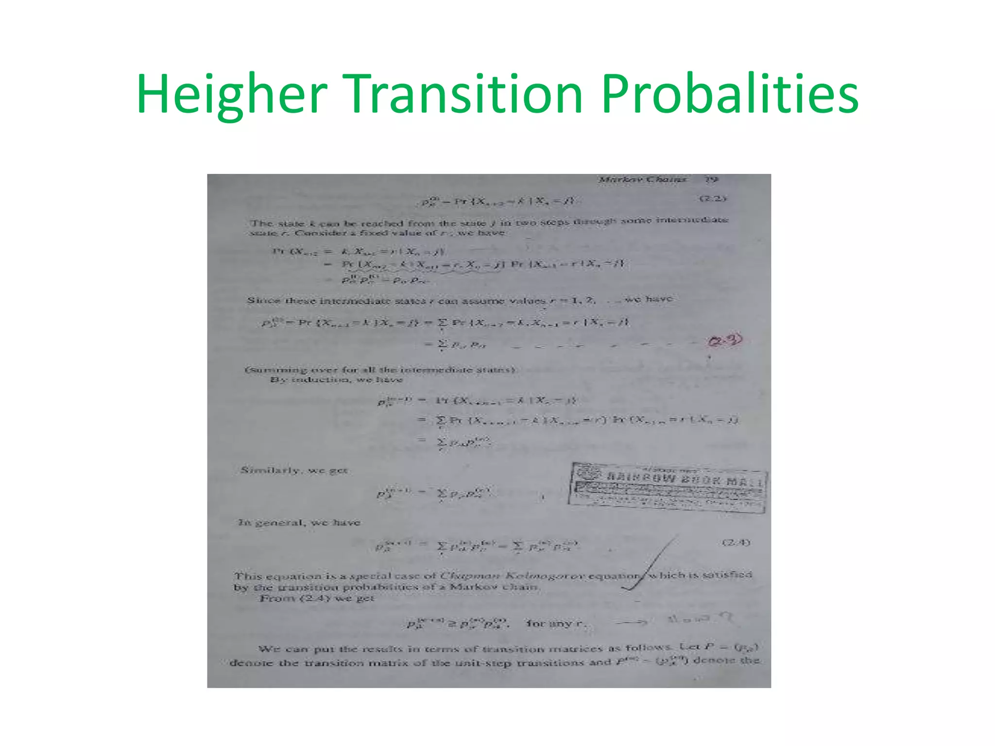
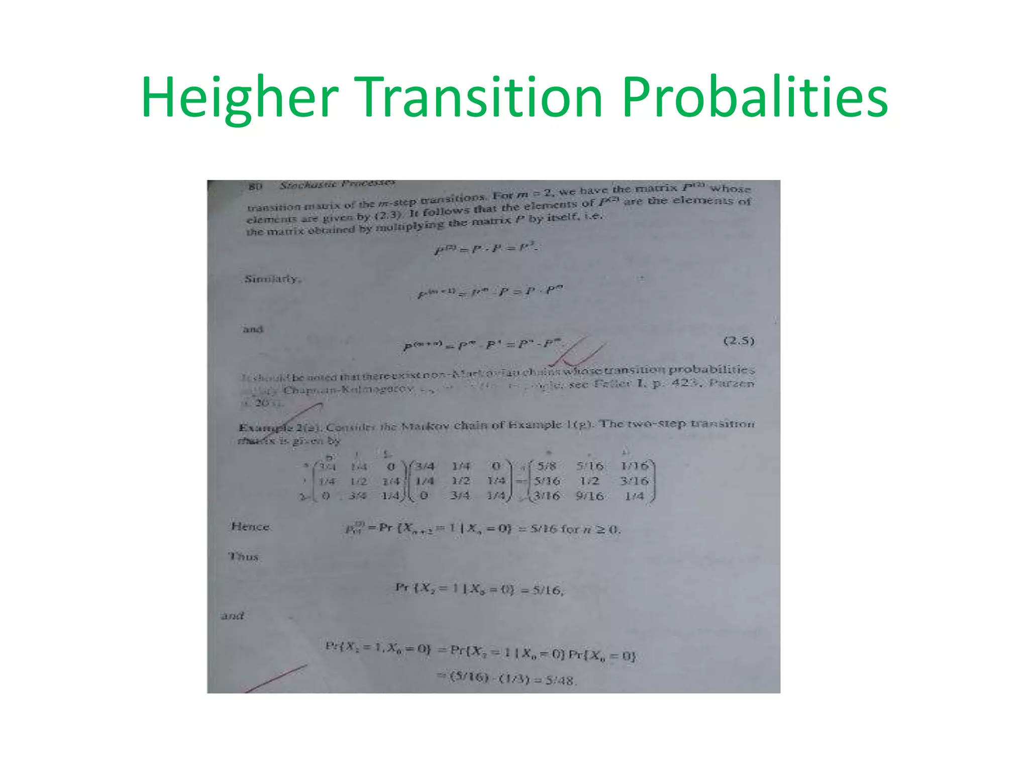
Exploration of probability distribution relevant to Markov chains, outlining fundamental concepts.
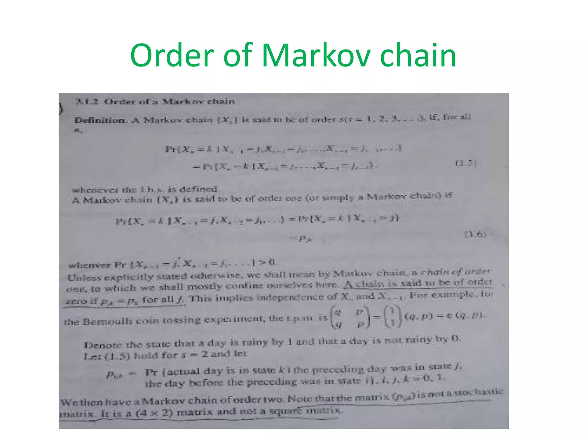
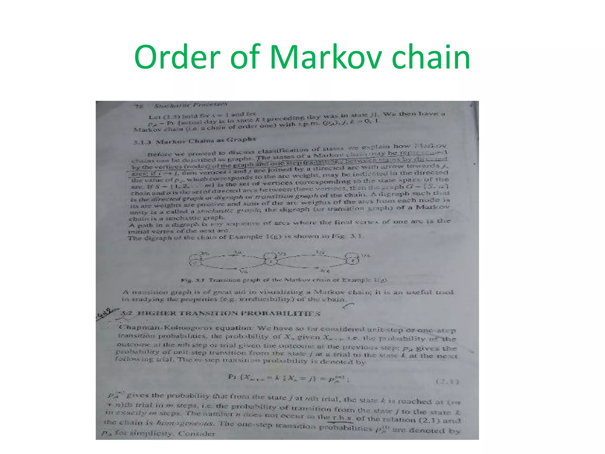
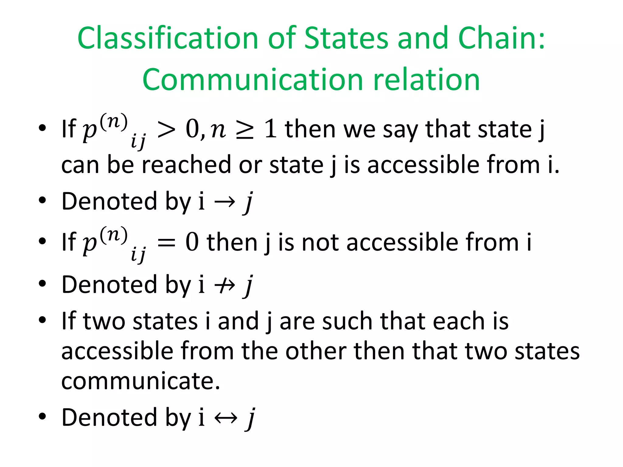
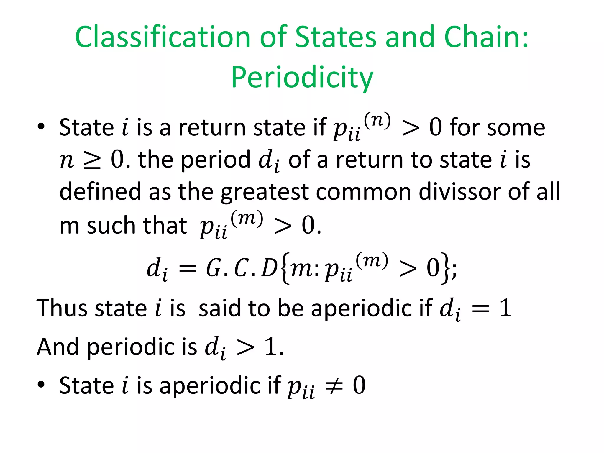
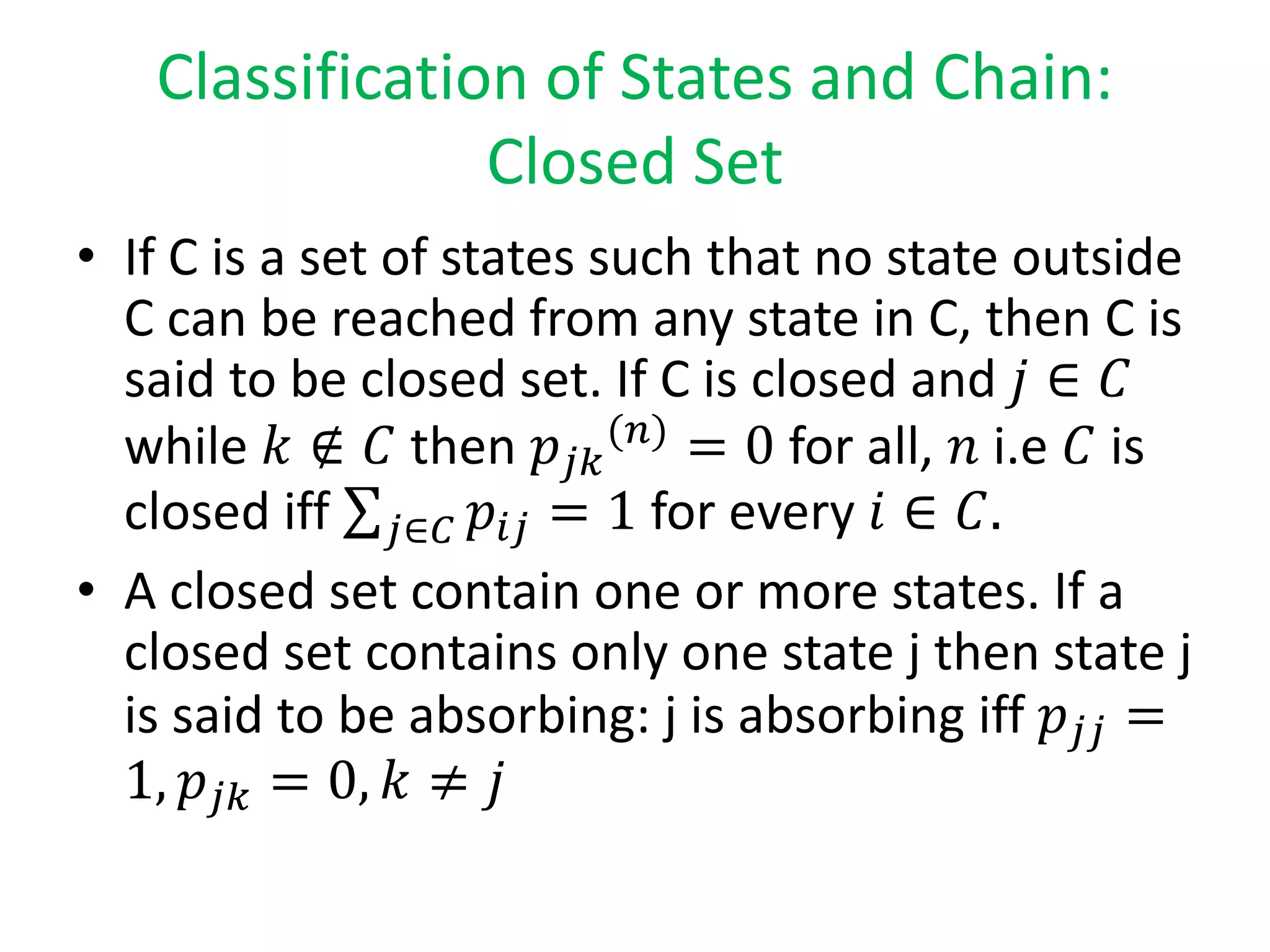
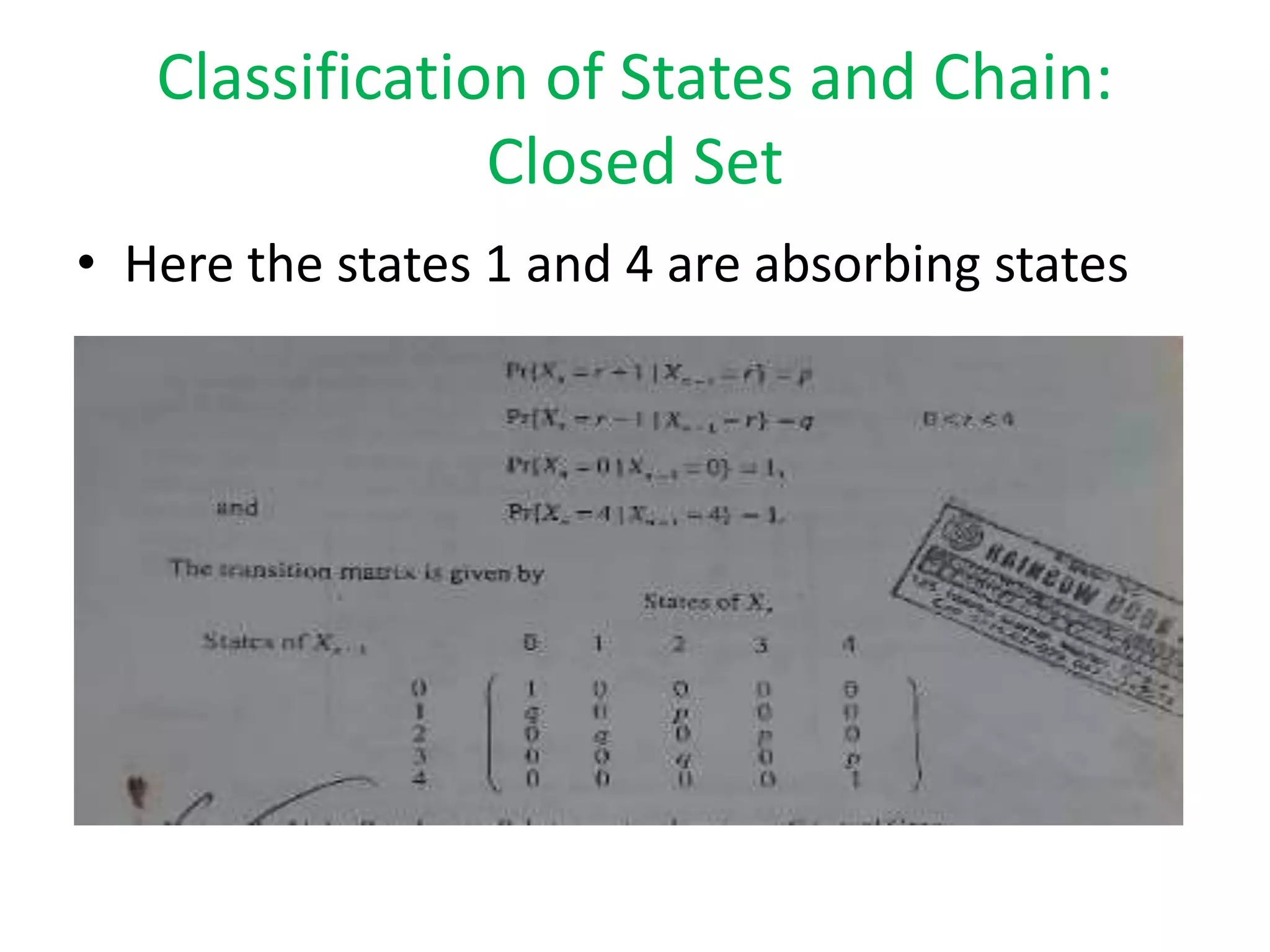
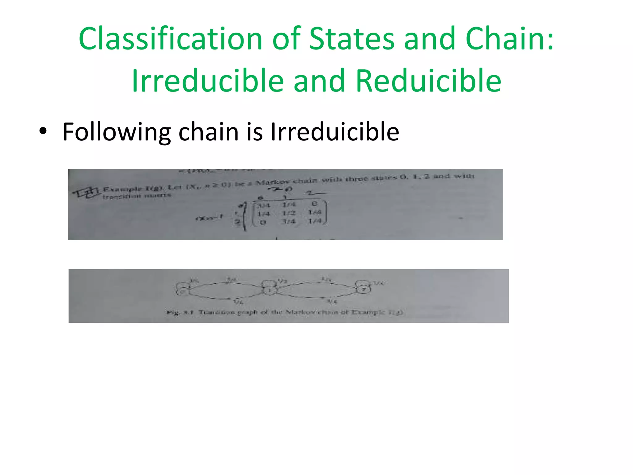
Detailed classification of states in Markov chains including communication relations, periodicity, and reducibility.
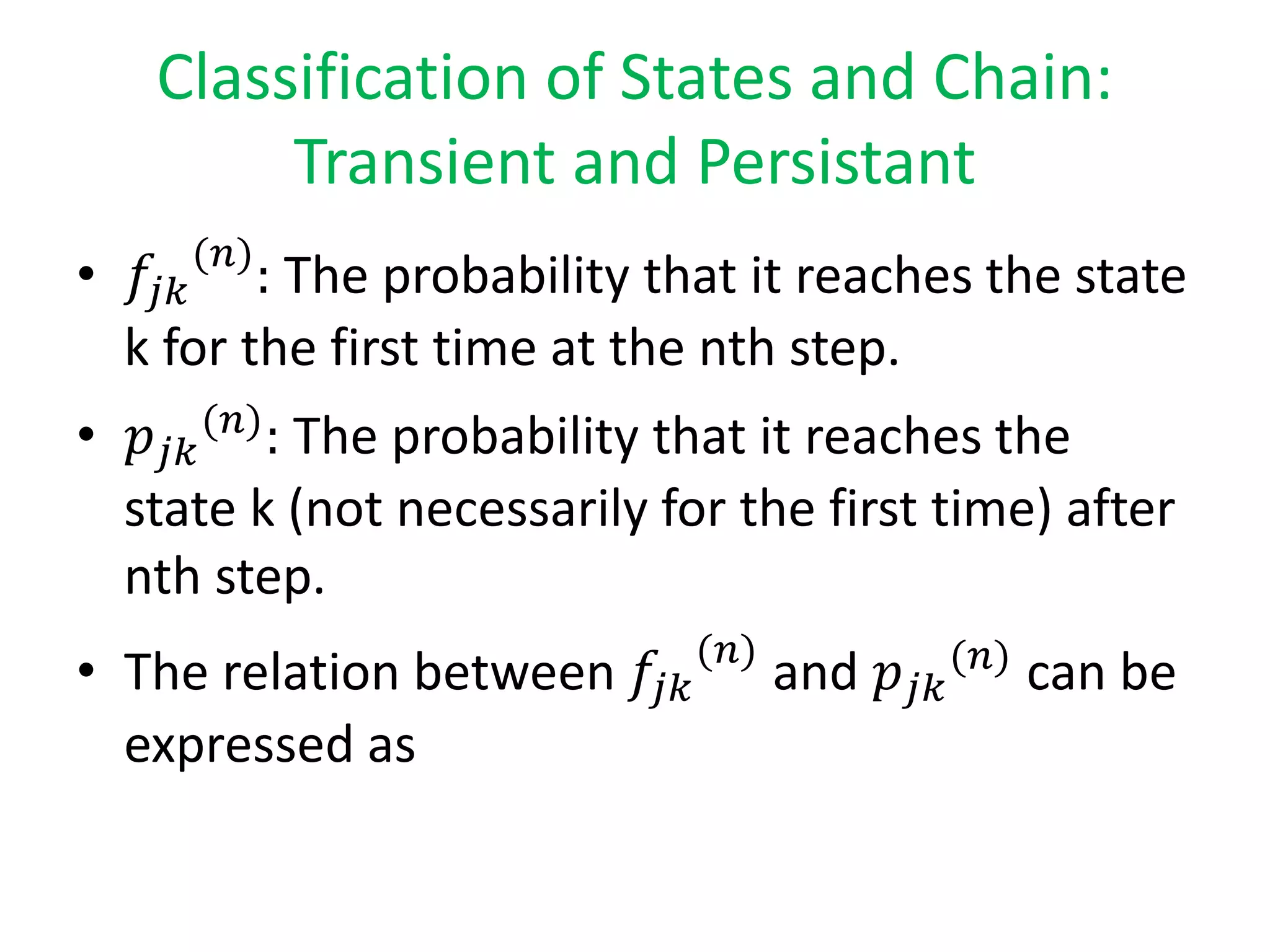
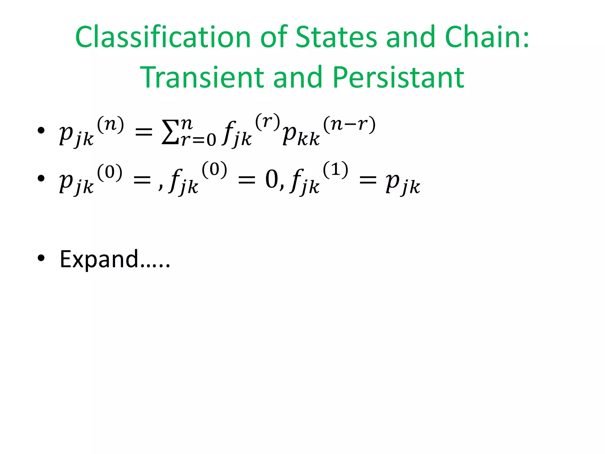
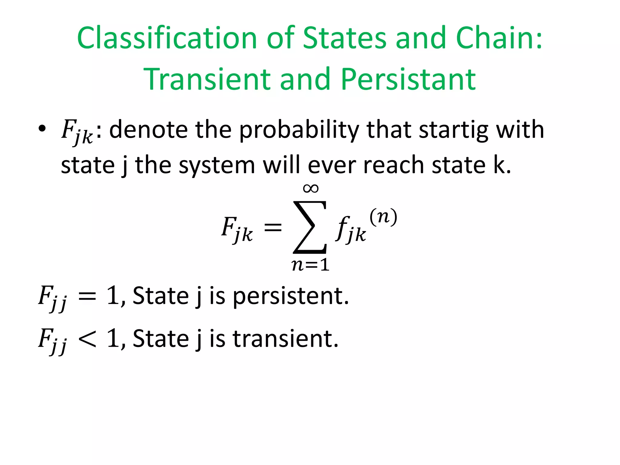
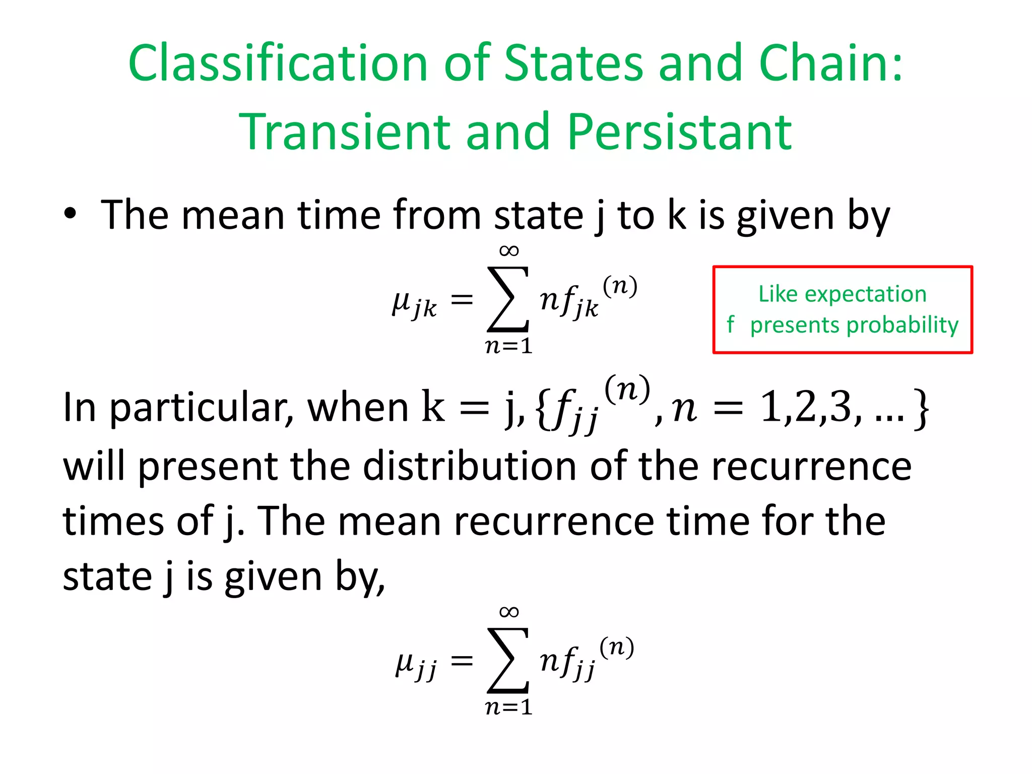
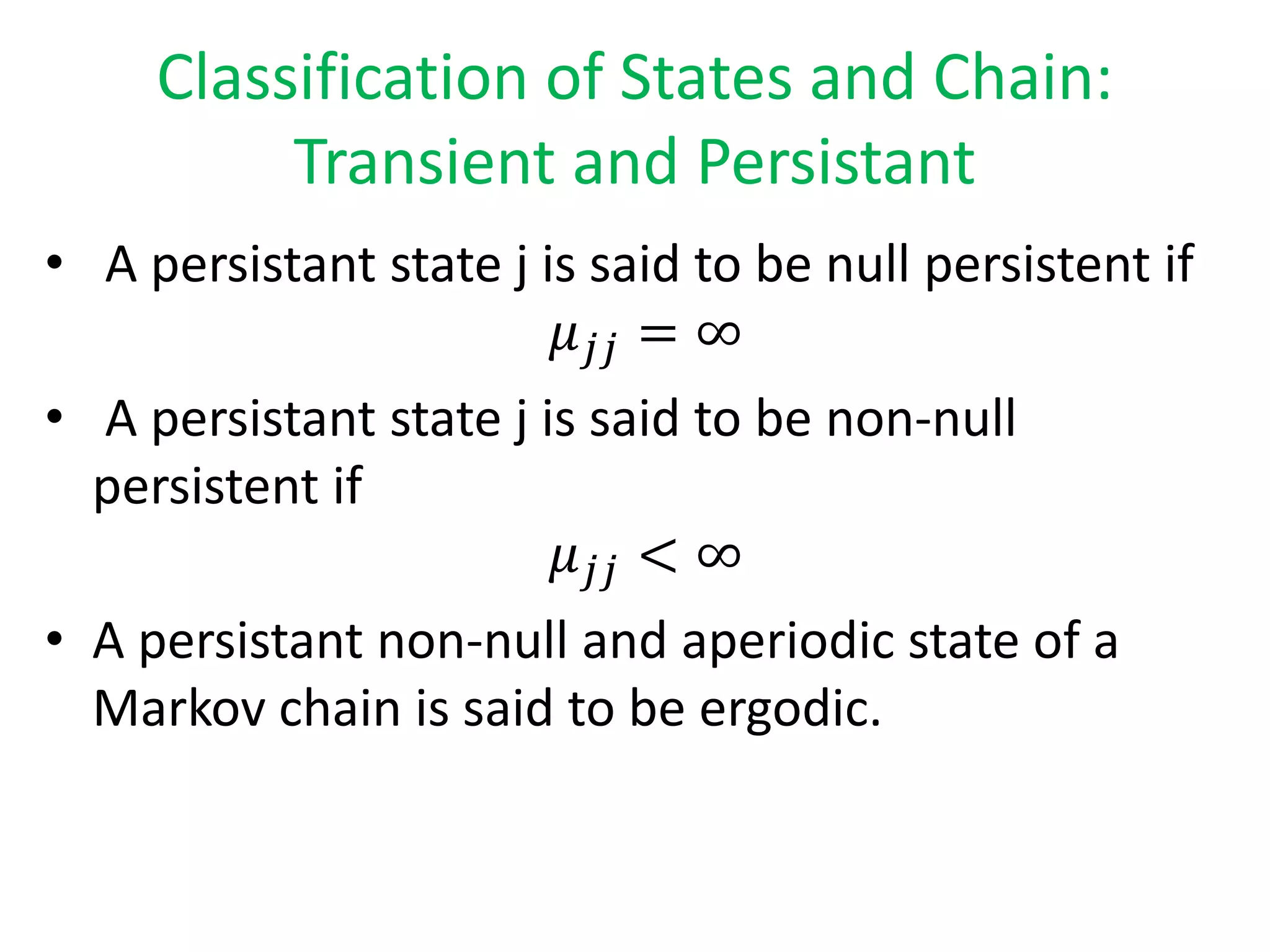
Examines transient and persistent states in Markov chains, focusing on transition probabilities and recurrent times.


![[DSC Europe 25] Debmalya Biswas - Agentification: the art of transforming man...](https://cdn.slidesharecdn.com/ss_thumbnails/r5azlggvtqiaiiusrqdr-4-251212103249-5a12c89b-thumbnail.jpg?width=640&height=640&fit=bounds)
![[DSC Europe 25] Branko Dzakula - From Defense to Attack: How AI Redefines Cyb...](https://cdn.slidesharecdn.com/ss_thumbnails/80bdzdxpr3ky2g0qvyk9-8-251211083048-ce5fc1ee-thumbnail.jpg?width=640&height=640&fit=bounds)
![[DSC Europe 25] Dusan Nesic - Securing Tomorrow’s Infrastructure: Why Cyber-P...](https://cdn.slidesharecdn.com/ss_thumbnails/qikbszfftyowjm2q6duw-1-251211083848-8f2ead6b-thumbnail.jpg?width=640&height=640&fit=bounds)
![[DSC Europe 25] Milan Zdravkovic - The road less traveled in District Heating...](https://cdn.slidesharecdn.com/ss_thumbnails/nfaboniqwsz4ucyctnmy-2-milan-zdravkovic-dsc2025-the-road-less-traveled-in-district-heating-operation-251208151905-f56388a5-thumbnail.jpg?width=640&height=640&fit=bounds)
![[DSC Europe 25] Dusan Pavlov - There Is No Spoon: Inferring Vision from Neura...](https://cdn.slidesharecdn.com/ss_thumbnails/wg0v1umoqjm4nnbd3p0v-there-is-no-spoon-251205085715-6d81d6c5-thumbnail.jpg?width=640&height=640&fit=bounds)


![[DSC Europe 25] Imai Jen-La Plante - The New Generation: AI and the Future of...](https://cdn.slidesharecdn.com/ss_thumbnails/kxi8t2l5rggivgcenyba-1-jenlaplante-dsc-251208152532-d1e076c2-thumbnail.jpg?width=640&height=640&fit=bounds)

![[DSC Europe 25] Aleksandra Dragicevic - AI-Boosted Research in Healthcare: Fr...](https://cdn.slidesharecdn.com/ss_thumbnails/iqwngszurf2r7pi1lnnj-4-aleksandra-dragicevic-ad-dsc-europe-conference-20-251208151905-37c3238a-thumbnail.jpg?width=640&height=640&fit=bounds)
![[DSC Europe 25] Sara Polak - The Ancient Operating System: What Archaeology T...](https://cdn.slidesharecdn.com/ss_thumbnails/3vch2p6tttdnwhsgazoz-3-sara-polak-smart-cities-251208152532-64404202-thumbnail.jpg?width=640&height=640&fit=bounds)

![[DSC Europe 25] Goran Obradovic - The Rise of Sovereign AI: Building the Regi...](https://cdn.slidesharecdn.com/ss_thumbnails/7nw2xxixrxqdxvrb5wca-6-251205085714-ab09a2ac-thumbnail.jpg?width=640&height=640&fit=bounds)

![[DSC Europe 25] Vladimir Jelic - The AI-Driven Security Shift From Reactive D...](https://cdn.slidesharecdn.com/ss_thumbnails/6g5gj25mtjwayniqem1t-6-251209104645-7a5a5fc6-thumbnail.jpg?width=640&height=640&fit=bounds)
![[DSC Europe 25] Dusan Jovicic - AI Story: From on-prem to cloud and back agai...](https://cdn.slidesharecdn.com/ss_thumbnails/8kp49m6uq22ifnbwhfnk-2-251205085715-964d11a6-thumbnail.jpg?width=640&height=640&fit=bounds)