Download as PDF, PPTX
![• Goal: Find the local minima !
𝒘 that are generalizable to test samples
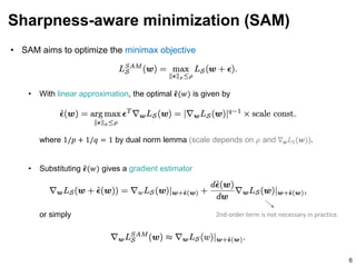
• Method: Minimize the sharpness-aware objective (SAM) instead of ERM
• “Flat minima” improves generalization (e.g., [1])
• With some approximation, SAM objective is computed by 2-step gradient descent
where !
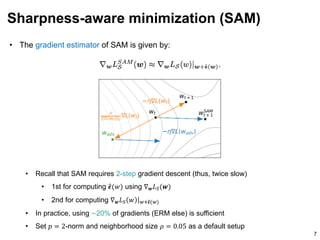
𝝐(𝒘) is a function of the gradient on original weights ∇𝒘𝐿"(𝒘)
• Results: Used for recent SOTA methods (e.g., NFNet [2], {ViT, MLP-Mixer}-SAM [3])
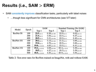
• SAM consistently improves classification tasks, particularly when with label noises
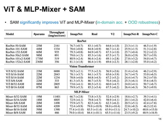
• With SAM, ViT outperforms ResNet of the same size (MLP-Mixer on par) – by [3]
1 minute summary
2
[1] Fantastic Generalization Measures and Where to Find Them. ICLR 2020.
[2] High-Performance Large-Scale Image Recognition Without Normalization. ICML 2021.
[3] When Vision Transformers Outperform ResNets without Pretraining or Strong Data Augmentations. Under review.](https://image.slidesharecdn.com/210616sam-210615200804/85/Sharpness-aware-minimization-SAM-2-320.jpg)
![• Given a training dataset 𝑆 from data distribution 𝒟, generalization bound aims to
guarantee the population loss 𝐿𝒟 with the sample loss 𝐿"
• Here, the gap of 𝐿𝒟 and 𝐿" is bounded by a function of complexity measure
• e.g., VC dimension, norm-based, distance from initialization, optimization-based
• In particular, the flatness-based measures correlate well with empirical results [1]
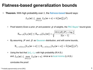
• Theorem. With high probability over 𝑆, the flatness-based bound says:
Flatness-based generalization bounds
4
Strictly increasing function of 𝒘.
Decreases as the number of
samples 𝑛 = 𝑆 increases.
[1] Fantastic Generalization Measures and Where to Find Them. ICLR 2020.](https://image.slidesharecdn.com/210616sam-210615200804/85/Sharpness-aware-minimization-SAM-4-320.jpg)
![• Loss surface visualization [1]
(two random directions)
• Hessian spectra
Verification of the flatness
8
[1] Visualizing the Loss Landscape of Neural Nets. NeurIPS 2018.
ERM SAM](https://image.slidesharecdn.com/210616sam-210615200804/85/Sharpness-aware-minimization-SAM-8-320.jpg)
![• Entropy-SGD [1] minimizes the local entropy near the weights
• Minimize average, not worst case of the neighborhood
• Stochastic weight averaging (SWA) [2] simply averages the intermediate weights
• Does not guarantee flat minima, but empirically works well
• Like the exponential weight averaging (EMA)
• Adversarial weight perturbation (AWP) [3] consider the similar idea of SAM, but
under the adversarial robustness setting
• Here, one can compute data and weight perturbations simultaneously
Some related works
10
[1] Entropy-SGD: Biasing Gradient Descent Into Wide Valleys. ICLR 2017.
[2] Averaging Weights Leads to Wider Optima and Better Generalization. UAI 2018.
[3] Adversarial Weight Perturbation Helps Robust Generalization. NeurIPS 2020.](https://image.slidesharecdn.com/210616sam-210615200804/85/Sharpness-aware-minimization-SAM-10-320.jpg)
![• Recall: Vision Transformer (ViT) [2] uses Transformer-only architecture
and MLP-Mixer [3] replace the Transformer with MLP layers
SAM for ViT (and MLP-Mixer)
11
[1] When Vision Transformers Outperform ResNets without Pretraining or Strong Data Augmentations. Under review.
[2] An Image is Worth 16x16 Words: Transformers for Image Recognition at Scale. ICLR 2021.
[3] MLP-Mixer: An all-MLP Architecture for Vision. Under review.
The contents afterward
are from [1]
MLP-Mixer: patch-wise MLP + channel-wise MLP](https://image.slidesharecdn.com/210616sam-210615200804/85/Sharpness-aware-minimization-SAM-11-320.jpg)
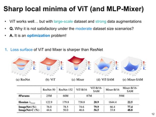
![• ViT works well… but with large-scale dataset and strong data augmentations
• Q. Why it is not satisfactory under the moderate dataset size scenarios?
• A. It is an optimization problem!
2. The training curves of ViT are often unstable [1]
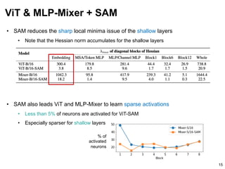
• Especially the shallow layers (e.g., embedding) are unstable
Sharp local minima of ViT (and MLP-Mixer)
13
[1] An Empirical Study of Training Self-Supervised Vision Transformers. Under review.
Accuracy dips Gradient spikes](https://image.slidesharecdn.com/210616sam-210615200804/85/Sharpness-aware-minimization-SAM-13-320.jpg)

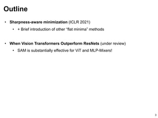
The document discusses the sharpness-aware minimization (SAM) technique, which enhances generalization in models by optimizing local minima that are flatter. It highlights the effectiveness of SAM, particularly with vision transformers (ViTs) and MLP mixers, demonstrating improvements in classification tasks and robustness against label noise. SAM consistently outperforms traditional empirical risk minimization in various scenarios, particularly for moderate dataset sizes.


![[DL輪読会]GLIDE: Guided Language to Image Diffusion for Generation and Editing](https://cdn.slidesharecdn.com/ss_thumbnails/glide2-220107030326-thumbnail.jpg?width=640&height=640&fit=bounds)