Download as PDF, PPTX


![Motivation [0]
• As shown in his paper in 1906, Markov’s original
motivation is purely mathematical:
– Application of The Weak Law of Large Number to dependent
random variables.
• However, we shall not follow this motivation...
28/03/2011 Markov models 4](https://image.slidesharecdn.com/hmmrevisited-110329122929-phpapp02/85/Markov-Models-4-320.jpg)
![Motivation [1]
• From the viewpoint of classification:
– Context-free classification: Bayes classifier
p (ωi | x ) > p (ω j | x ) ∀j ≠ i
28/03/2011 Markov models 5](https://image.slidesharecdn.com/hmmrevisited-110329122929-phpapp02/85/Markov-Models-5-320.jpg)
![Motivation [1]
• From the viewpoint of classification:
– Context-free classification: Bayes classifier
p (ωi | x ) > p (ω j | x ) ∀j ≠ i
• Classes are independent.
• Feature vectors are independent.
28/03/2011 Markov models 6](https://image.slidesharecdn.com/hmmrevisited-110329122929-phpapp02/85/Markov-Models-6-320.jpg)
![Motivation [1]
• From the viewpoint of classification:
– Context-free classification: Bayes classifier
p (ωi | x ) > p (ω j | x ) ∀j ≠ i
– However, there are some applications where various
classes are closely realated:
• POS Tagging, Tracking, Gene boundary recover...
s1 s2 s3 ... sm ...
28/03/2011 Markov models 7](https://image.slidesharecdn.com/hmmrevisited-110329122929-phpapp02/85/Markov-Models-7-320.jpg)
![Motivation [1]
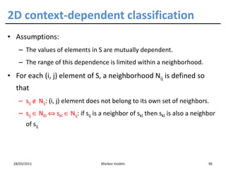
• Context-dependent classification:
s1 s2 s3 ... sm ...
– s1, s2, ..., sm: sequence of m feature vector
– ω1, ω2,..., ωN: classes in which these vectors are classified: ωi = 1...k.
28/03/2011 Markov models 8](https://image.slidesharecdn.com/hmmrevisited-110329122929-phpapp02/85/Markov-Models-8-320.jpg)
![Motivation [1]
• Context-dependent classification:
s1 s2 s3 ... sm ...
– s1, s2, ..., sm: sequence of m feature vector
– ω1, ω2,..., ωN: classes in which these vectors are classified: ωi = 1...k.
• To apply Bayes classifier:
– X = s1s2...sm: extened feature vector
– Ωi = ωi1, ωi2,..., ωiN : a classification Nm possible classifications
p ( Ωi | X ) > p ( Ω j | X ) ∀j ≠ i
p ( X | Ωi ) p ( Ωi ) > p ( X | Ω j ) p ( Ω j ) ∀j ≠ i
28/03/2011 Markov models 9](https://image.slidesharecdn.com/hmmrevisited-110329122929-phpapp02/85/Markov-Models-9-320.jpg)
![Motivation [1]
• Context-dependent classification:
s1 s2 s3 ... sm ...
– s1, s2, ..., sm: sequence of m feature vector
– ω1, ω2,..., ωN: classes in which these vectors are classified: ωi = 1...k.
• To apply Bayes classifier:
– X = s1s2...sm: extened feature vector
– Ωi = ωi1, ωi2,..., ωiN : a classification Nm possible classifications
p ( Ωi | X ) > p ( Ω j | X ) ∀j ≠ i
p ( X | Ωi ) p ( Ωi ) > p ( X | Ω j ) p ( Ω j ) ∀j ≠ i
28/03/2011 Markov models 10](https://image.slidesharecdn.com/hmmrevisited-110329122929-phpapp02/85/Markov-Models-10-320.jpg)
![Motivation [2]
• From a general view, sometimes we want to evaluate the joint
distribution of a sequence of dependent random variables
28/03/2011 Markov models 11](https://image.slidesharecdn.com/hmmrevisited-110329122929-phpapp02/85/Markov-Models-11-320.jpg)
![Motivation [2]
• From a general view, sometimes we want to evaluate the joint
distribution of a sequence of dependent random variables
Hôm nay mùng tám tháng ba
Chị em phụ nữ đi ra đi vào...
Hôm nay mùng ... vào ...
q1 q2 q3 qm
28/03/2011 Markov models 12](https://image.slidesharecdn.com/hmmrevisited-110329122929-phpapp02/85/Markov-Models-12-320.jpg)
![Motivation [2]
• From a general view, sometimes we want to evaluate the joint
distribution of a sequence of dependent random variables
Hôm nay mùng tám tháng ba
Chị em phụ nữ đi ra đi vào...
Hôm nay mùng ... vào ...
q1 q2 q3 qm
• What is p(Hôm nay.... vào) = p(q1=Hôm q2=nay ... qm=vào)?
28/03/2011 Markov models 13](https://image.slidesharecdn.com/hmmrevisited-110329122929-phpapp02/85/Markov-Models-13-320.jpg)
![Motivation [2]
• From a general view, sometimes we want to evaluate the joint
distribution of a sequence of dependent random variables
Hôm nay mùng tám tháng ba
Chị em phụ nữ đi ra đi vào...
Hôm nay mùng ... vào ...
q1 q2 q3 qm
• What is p(Hôm nay.... vào) = p(q1=Hôm q2=nay ... qm=vào)?
p(s1s2... sm-1 sm)
p(sm|s1s2...sm-1) =
p(s1s2... sm-1)
28/03/2011 Markov models 14](https://image.slidesharecdn.com/hmmrevisited-110329122929-phpapp02/85/Markov-Models-14-320.jpg)


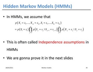
![Independence Assumptions in HMMs [1]
p ( ABC ) = p ( A | BC ) p ( BC ) = p ( A | BC ) p ( B ˚ C ) p ( C )
• By the chain rule, the following equality is exact:
p ( X 1 = x1 ,..., X m = xm , S1 = s1 ,..., S m = sm )
= p ( S1 = s1 ,..., S m = sm ) ×
p ( X 1 = x1 ,..., X m = xm ˚ S1 = s1 ,..., S m = sm )
• Assumption 1: the state sequence forms a Markov chain
m
p ( S1 = s1 ,..., S m = sm ) = p ( S1 = s1 ) ∏ p ( S j = s j ˚ S j −1 = s j −1 )
j =2
28/03/2011 Markov models 40](https://image.slidesharecdn.com/hmmrevisited-110329122929-phpapp02/85/Markov-Models-40-320.jpg)
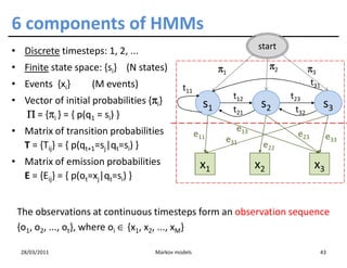
![Independence Assumptions in HMMs [2]
• By the chain rule, the following equality is exact:
p ( X 1 = x1 ,..., X m = xm ˚ S1 = s1 ,..., S m = sm )
m
= ∏ p ( X j = x j ˚ S1 = s1 ,..., Sm = sm , X 1 = x1 ,..., X j −1 = x j −1 )
j =1
• Assumption 2: each observation depends only on the underlying
state
p ( X j = x j ˚ S1 = s1 ,..., Sm = sm , X 1 = x1 ,..., X j −1 = x j −1 )
= p( X j = xj ˚ S j = sj )
• These two assumptions are often called independence
assumptions in HMMs
28/03/2011 Markov models 41](https://image.slidesharecdn.com/hmmrevisited-110329122929-phpapp02/85/Markov-Models-41-320.jpg)


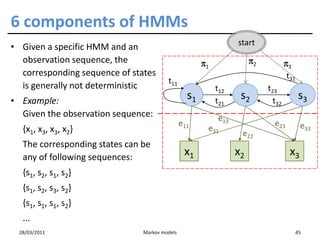


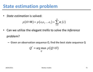


![Training HMMs
• Remember, we have just computed
p(o1o2...oT | Φ)
• Now, we have some observations and we want to inference Φ
from them.
• So, we could use:
– MAX LIKELIHOOD: Φ = arg max p ( o1 … oT | Φ )
Φ
– BAYES:
Compute p ( Φ | o1 … oT )
then take E [ Φ ] or max p ( Φ | o1 … oT )
Φ
28/03/2011 Markov models 82](https://image.slidesharecdn.com/hmmrevisited-110329122929-phpapp02/85/Markov-Models-82-320.jpg)


![MRF for Image Segmentation
• Gibbs distribution:
1 −U ( s )
π ( s ) = exp
Z T
– Z: normalizing constant
– T: parameter
• It turns out that Gibbs distribution implies MRF
([Gema 84])
28/03/2011 Markov models 101](https://image.slidesharecdn.com/hmmrevisited-110329122929-phpapp02/85/Markov-Models-101-320.jpg)
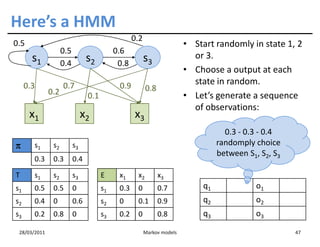
![MRF for Image Segmentation
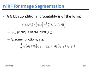
• Then, the joint probability for the Gibbs model is
∑∑ Fk ( Ck ( i, j ) )
i, j k
p ( S ) = exp −
T
– The sum is calculated over all possible cliques associated
with the neighborhood.
• We also need to work out p(X|S)
• Then p(X|S)p(S) can be maximized... [Gema 84]
28/03/2011 Markov models 103](https://image.slidesharecdn.com/hmmrevisited-110329122929-phpapp02/85/Markov-Models-103-320.jpg)
![What you should know
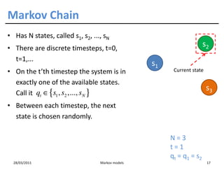
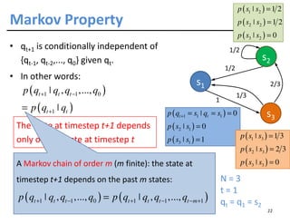
• Markov property, Markov Chain
• HMM:
– Defining and computing αt(i)
– Viterbi algorithm
– Outline of the EM algorithm for HMM
• Markov Random Field
– And an application in Image Segmentation
– [Geman 84] for more information.
28/03/2011 Markov models 105](https://image.slidesharecdn.com/hmmrevisited-110329122929-phpapp02/85/Markov-Models-105-320.jpg)


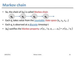
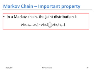
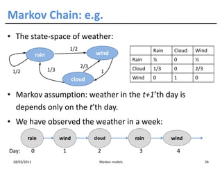
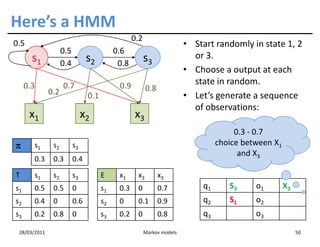
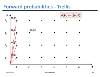
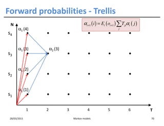
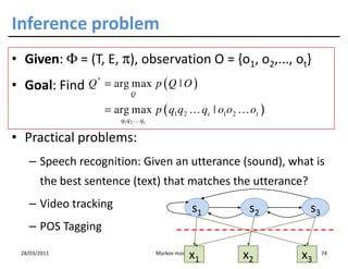
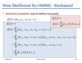
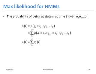
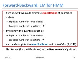
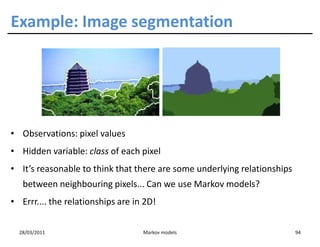
The document discusses Markov models, their origins from Andrei Markov, and applications across various fields such as natural language processing and bioinformatics. It explains concepts like Markov chains, Hidden Markov Models (HMMs), and the transition probabilities between states. The document highlights the importance of context-dependent classification in dealing with dependent random variables.