Downloaded 607 times
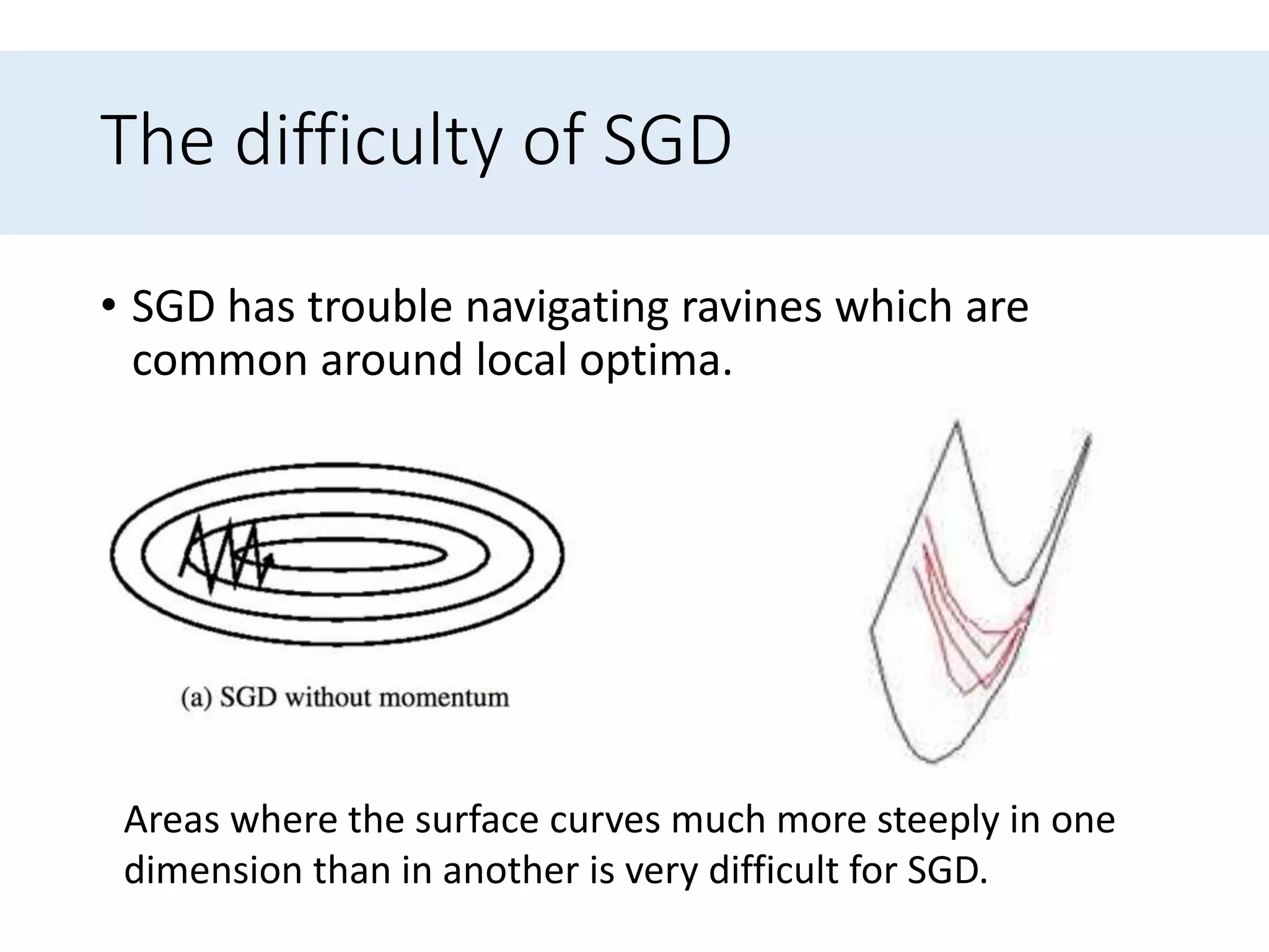
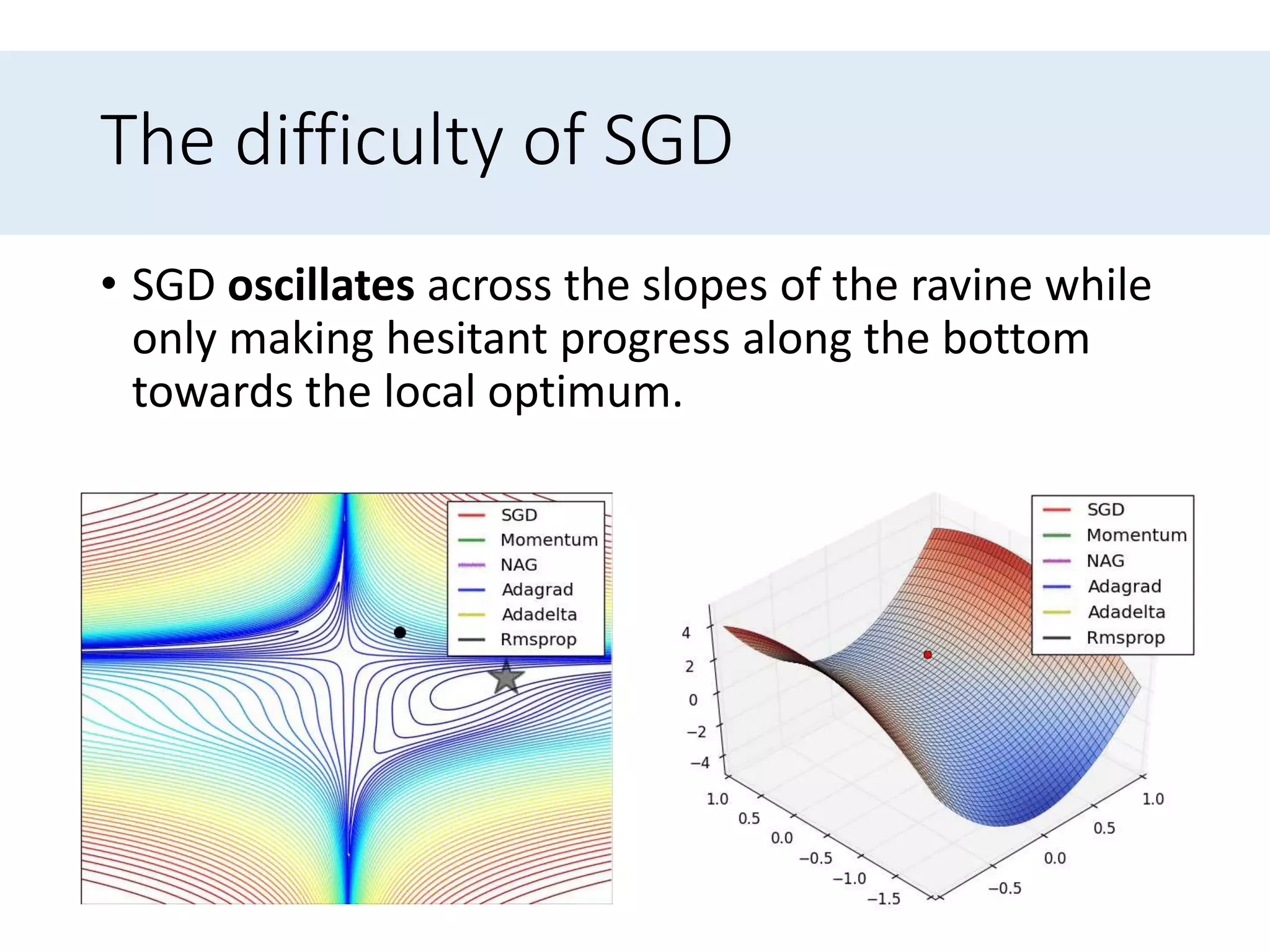
![Avoiding getting trapped in highly non-convex error
functions’ numerous suboptimal local minima
• Dauphin[5] argue that the difficulty arises in fact not
from local minima but from saddle points.
• Saddle points are at the places that one dimension slopes
up and another slopes down.
• These saddle points are usually surrounded by a
plateau of the same error as the gradient is close to
zero in all dimensions.
• This makes it hard for SGD to escape.
[5] Yann N. Dauphin, Razvan Pascanu, Caglar Gulcehre, Kyunghyun Cho, Surya Ganguli, and Yoshua Bengio. Identifying and
attacking the saddle point problem in high-dimensional nonconvex optimization. arXiv, pages 1–14, 2014.](https://image.slidesharecdn.com/anoverviewofgradientdescentoptimizationalgorithms-170414055411/75/An-overview-of-gradient-descent-optimization-algorithms-23-2048.jpg)

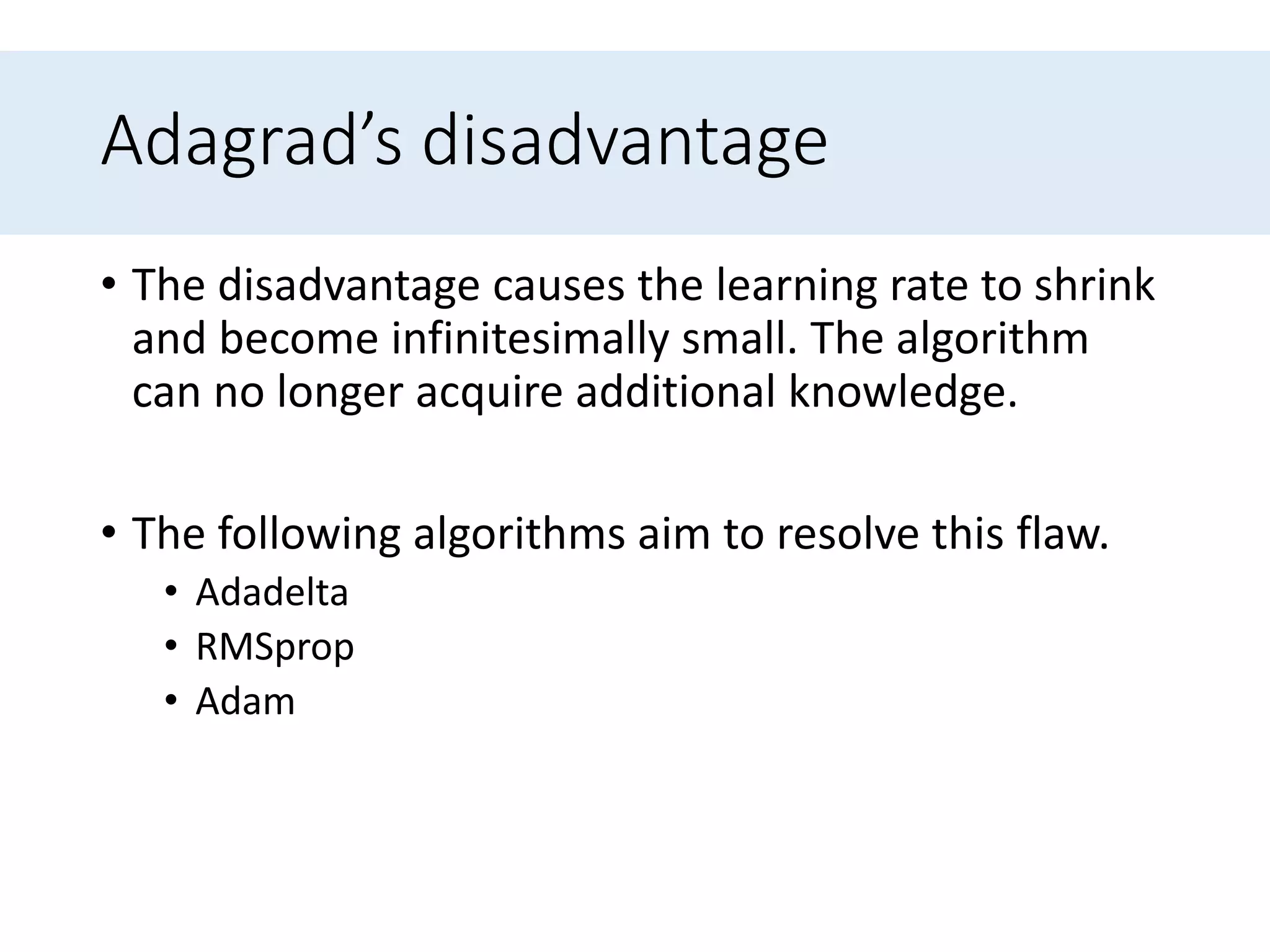
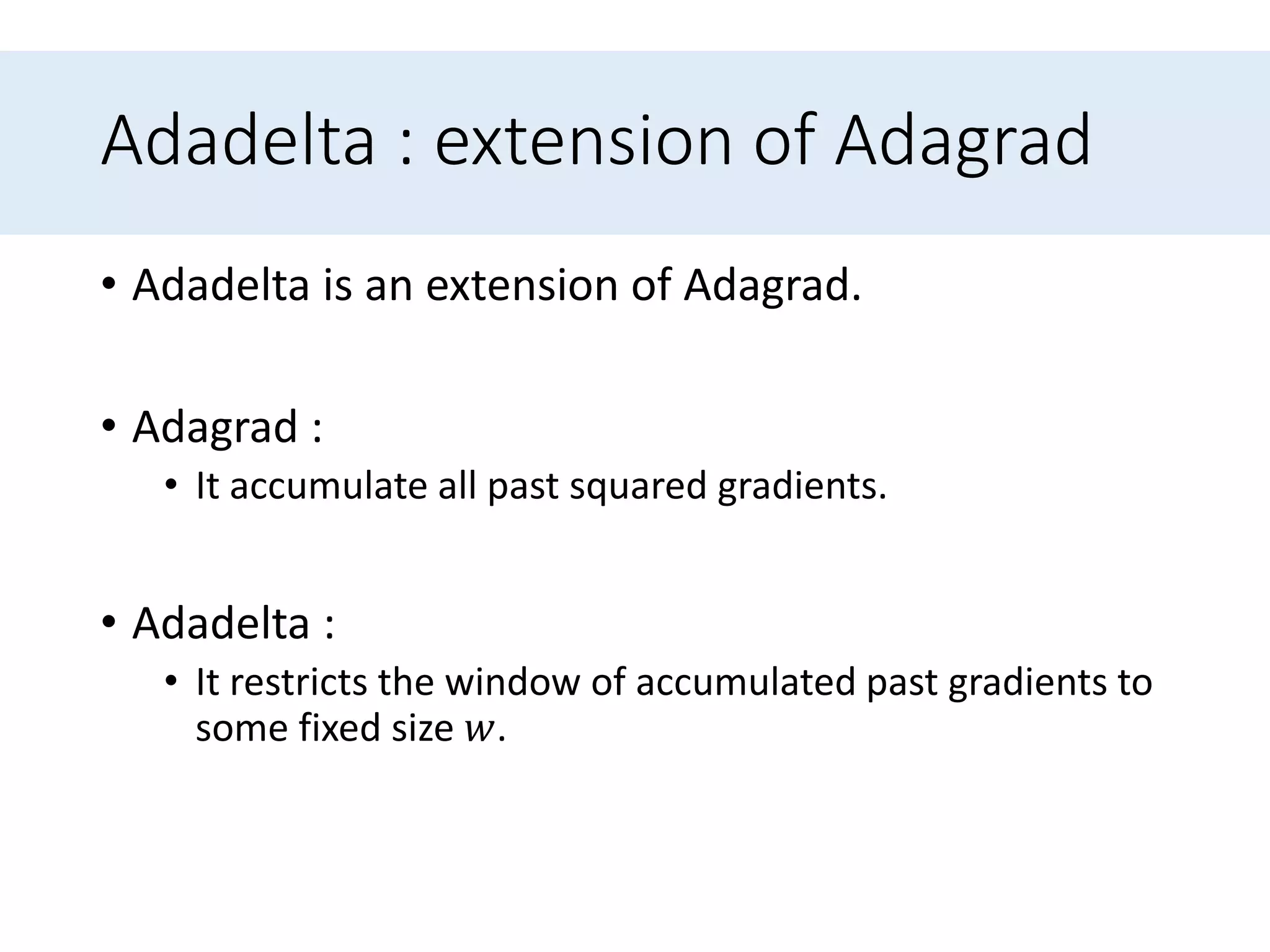
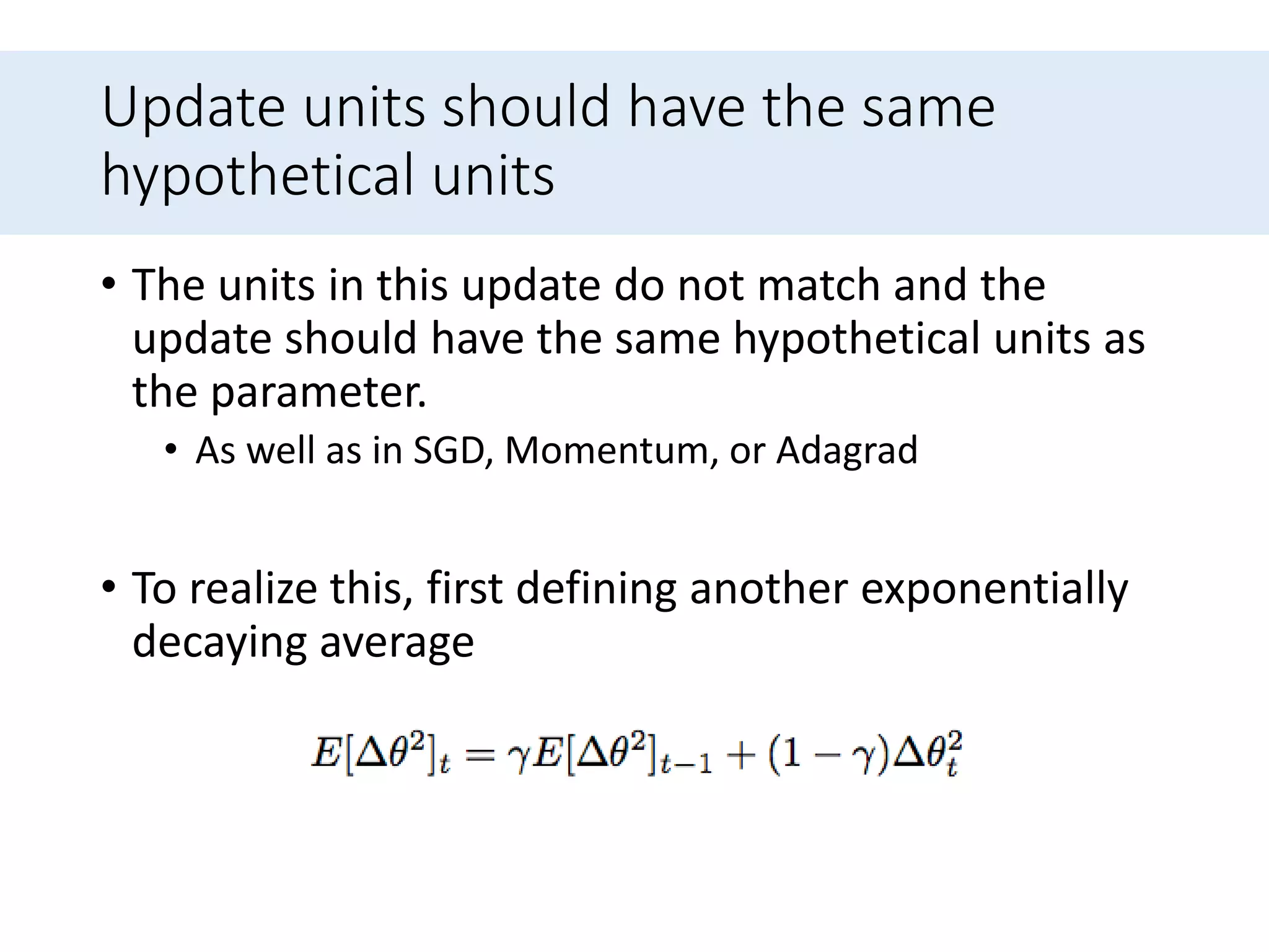
![Adadelta
• Instead of inefficiently storing, the sum of gradients
is recursively defined as a decaying average of all
past squared gradients.
• 𝐸[𝑔2] 𝑡 :The running average at time step 𝑡.
• 𝛾 : A fraction similarly to the Momentum term, around
0.9](https://image.slidesharecdn.com/anoverviewofgradientdescentoptimizationalgorithms-170414055411/75/An-overview-of-gradient-descent-optimization-algorithms-53-2048.jpg)
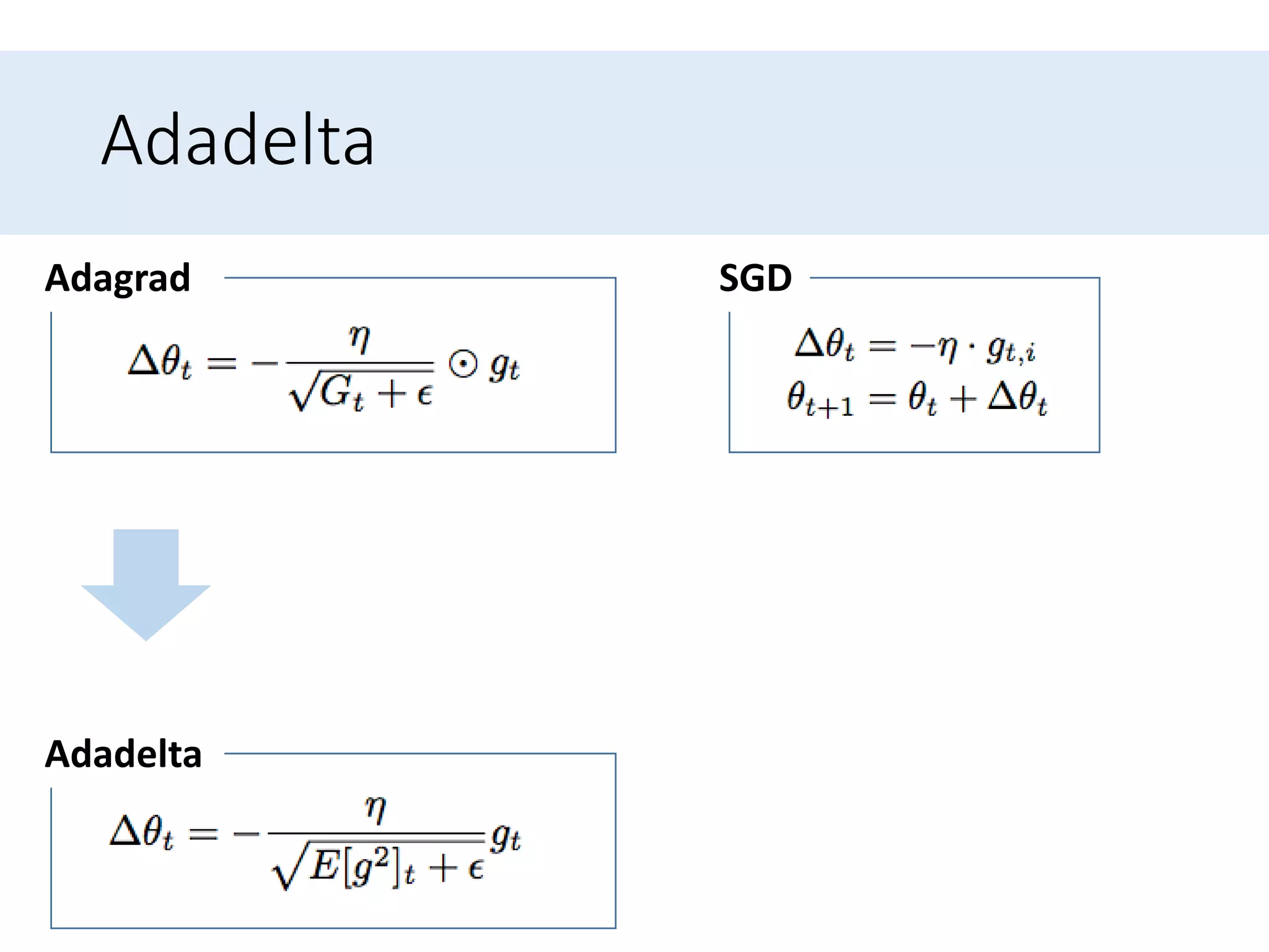
![Adadelta
SGDAdagrad
Adadelta
Replace the diagonal matrix 𝐺𝑡 with the decaying
average over past squared gradients 𝐸[𝑔2] 𝑡](https://image.slidesharecdn.com/anoverviewofgradientdescentoptimizationalgorithms-170414055411/75/An-overview-of-gradient-descent-optimization-algorithms-55-2048.jpg)
![Adadelta
SGDAdagrad
Adadelta Adadelta
Replace the diagonal matrix 𝐺𝑡 with the decaying
average over past squared gradients 𝐸[𝑔2] 𝑡](https://image.slidesharecdn.com/anoverviewofgradientdescentoptimizationalgorithms-170414055411/75/An-overview-of-gradient-descent-optimization-algorithms-56-2048.jpg)
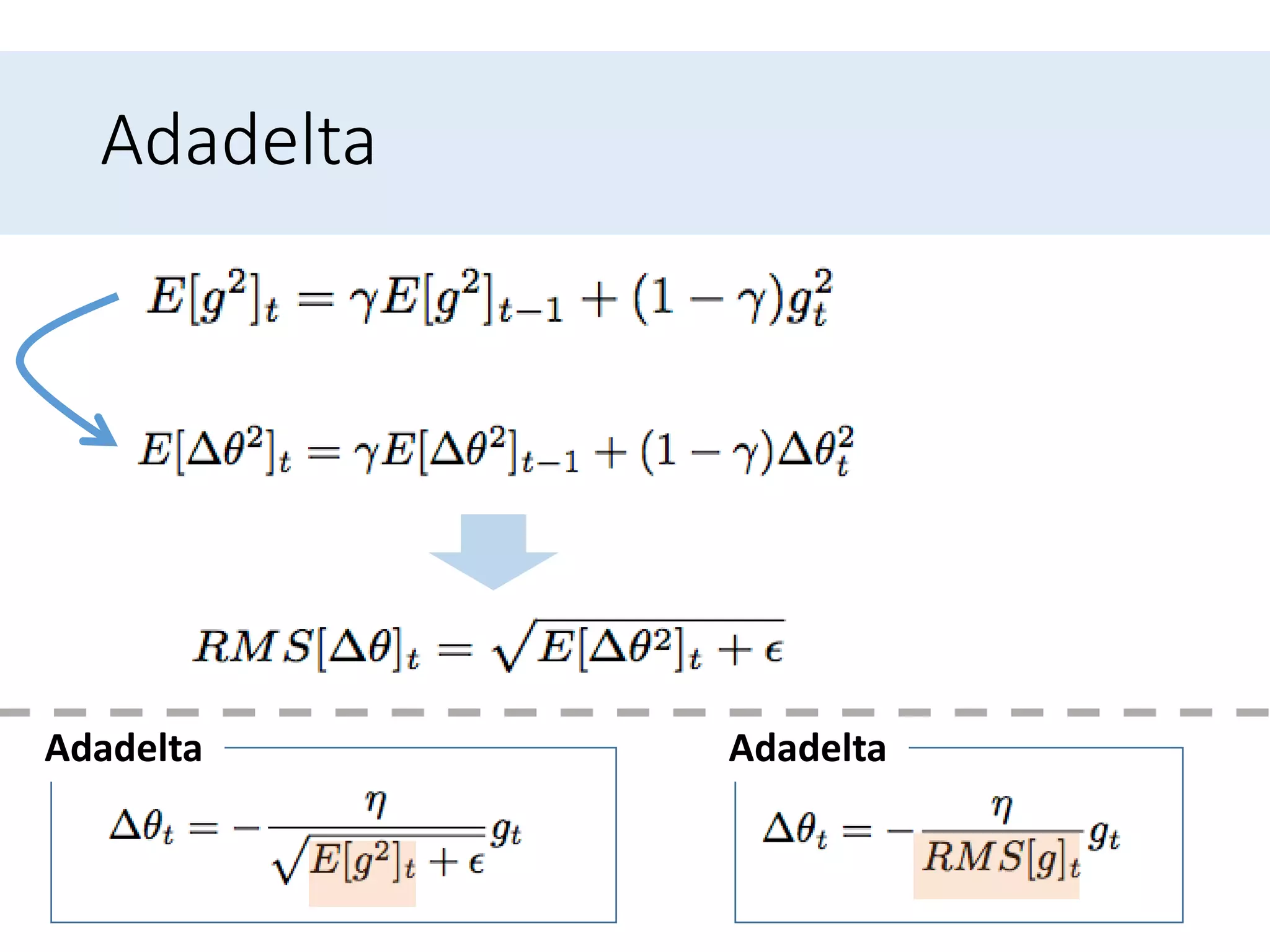
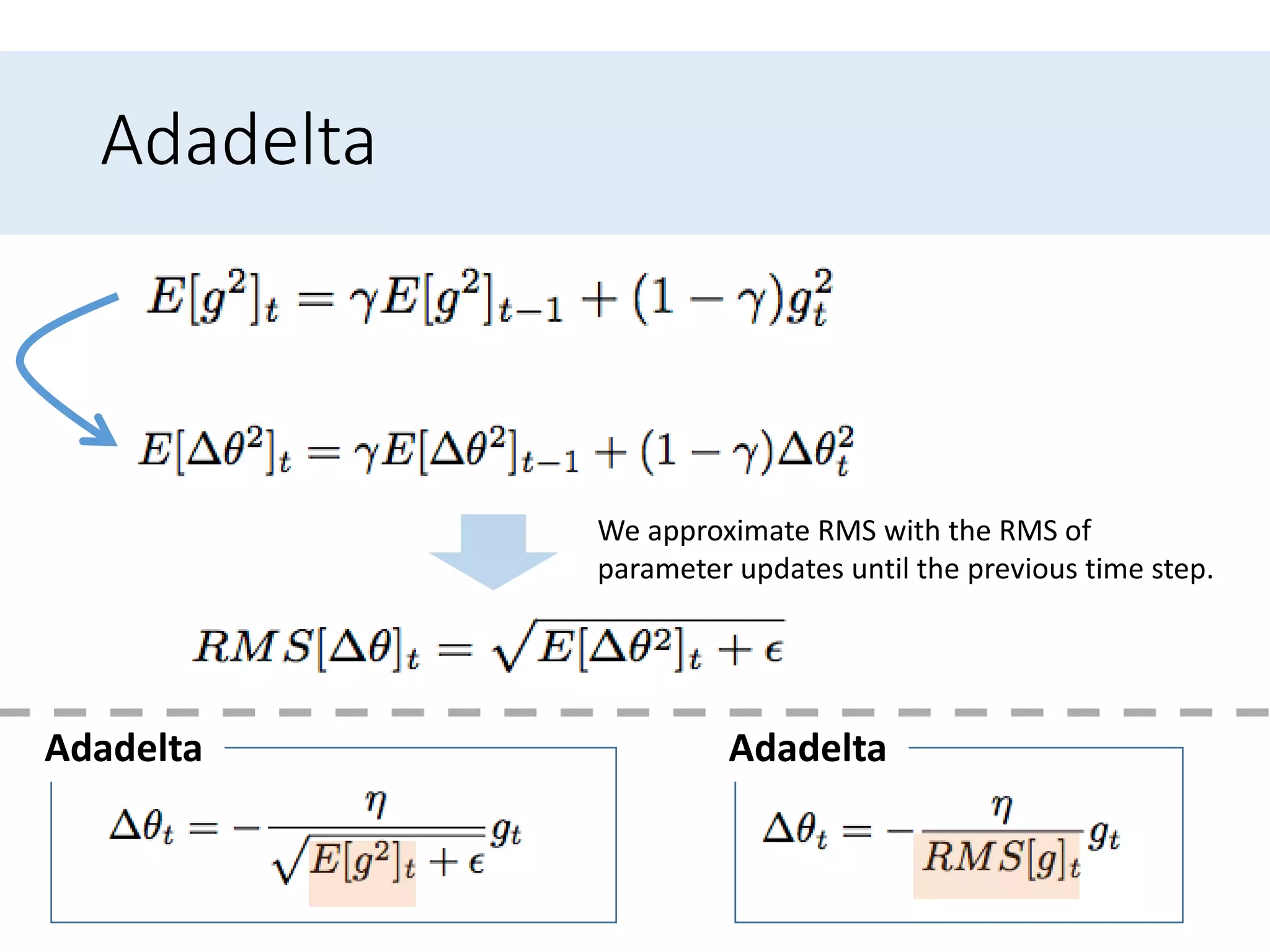
![Adadelta update rule
• Replacing the learning rate 𝜂 in the previous update
rule with 𝑅𝑀𝑆[∆𝜃] 𝑡−1 finally yields the Adadelta
update rule:
• Note : we do not even need to set a default
learning rate](https://image.slidesharecdn.com/anoverviewofgradientdescentoptimizationalgorithms-170414055411/75/An-overview-of-gradient-descent-optimization-algorithms-60-2048.jpg)
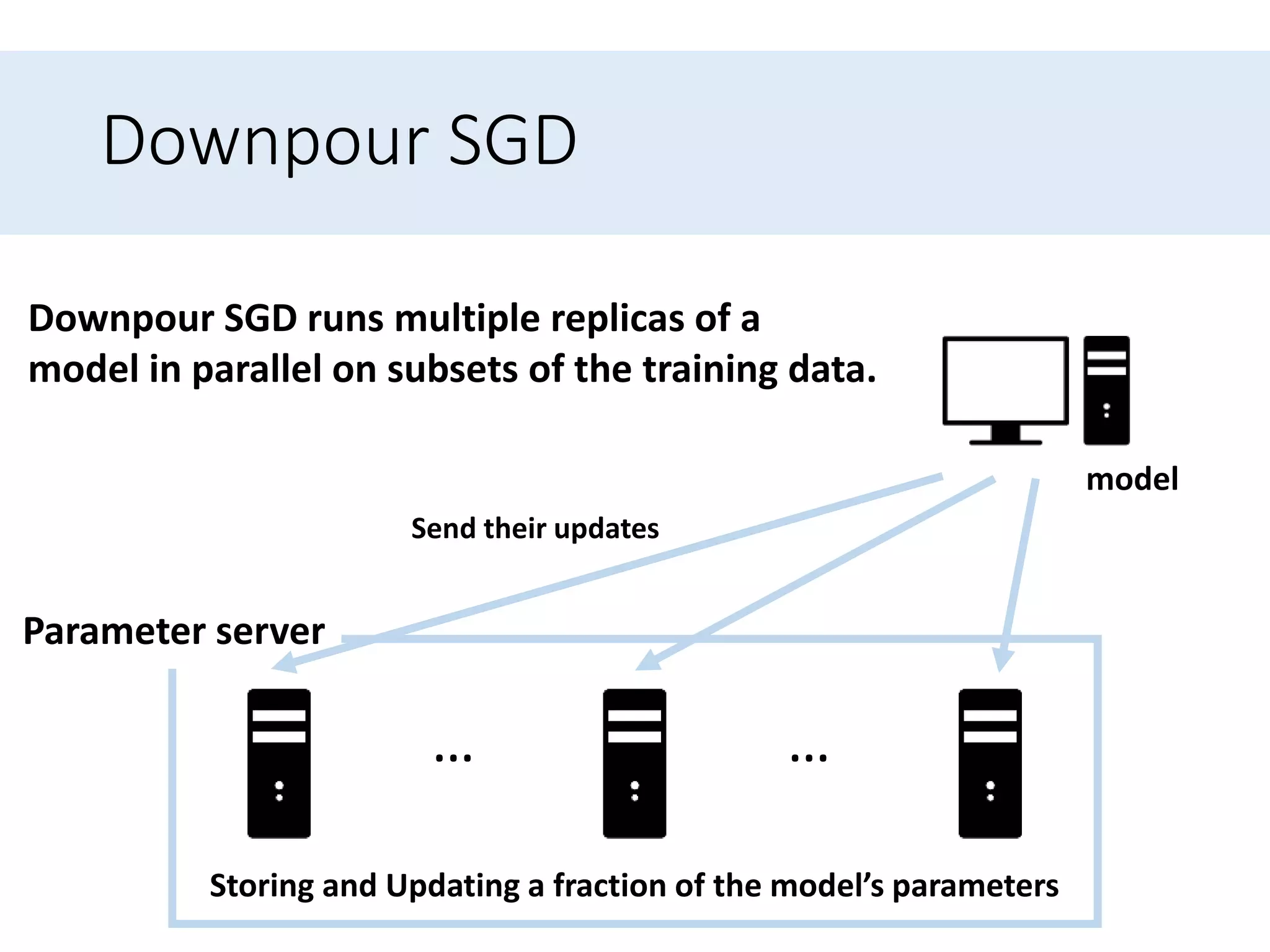
![Delay-tolerant Algorithms for SGD
• McMahan and Streeter [11] extend AdaGrad to the
parallel setting by developing delay-tolerant
algorithms that not only adapt to past gradients,
but also to the update delays.](https://image.slidesharecdn.com/anoverviewofgradientdescentoptimizationalgorithms-170414055411/75/An-overview-of-gradient-descent-optimization-algorithms-75-2048.jpg)
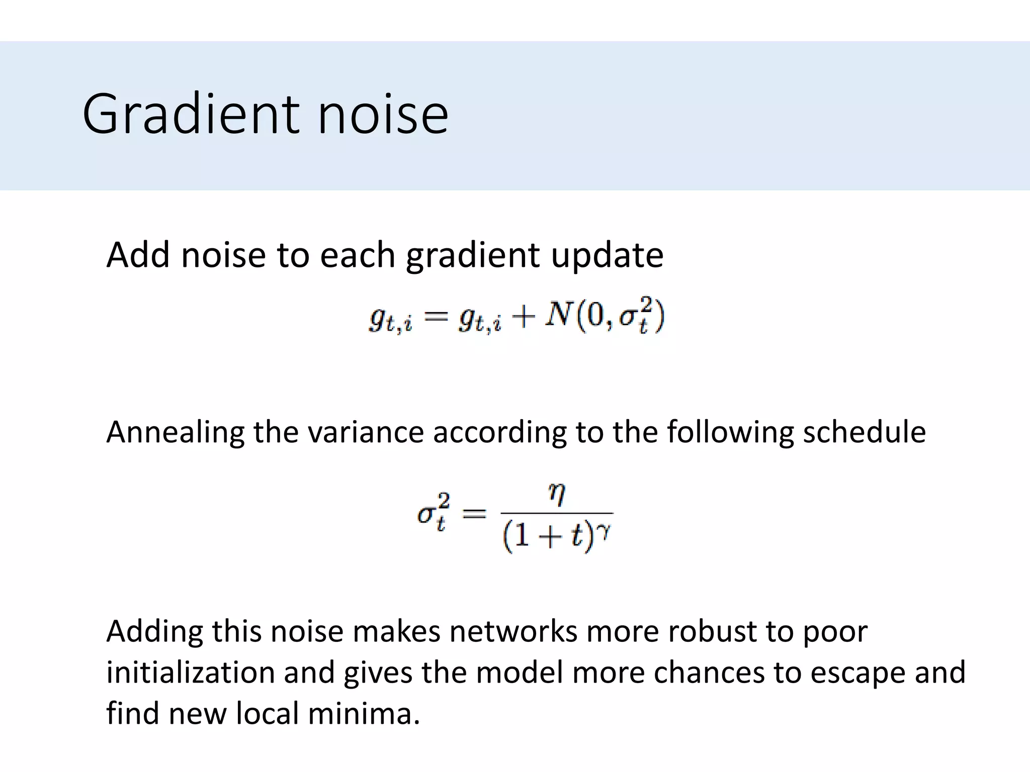


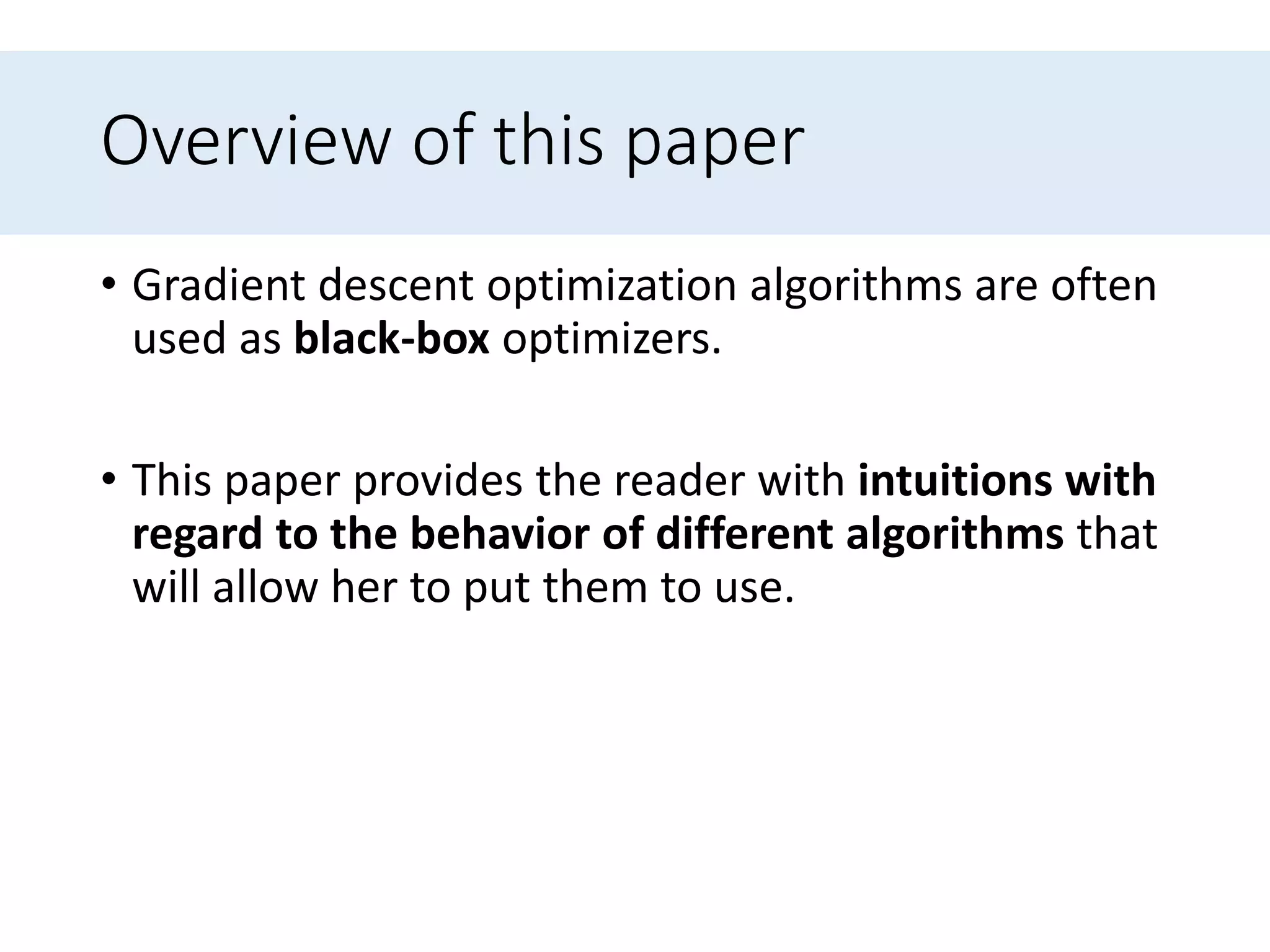
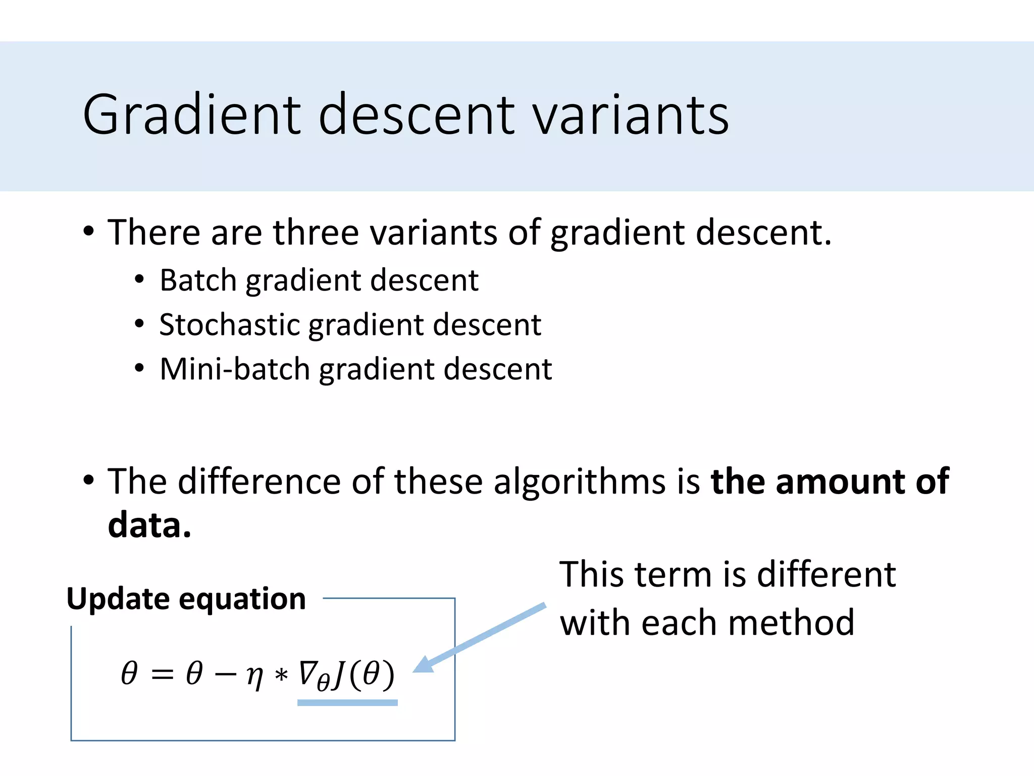
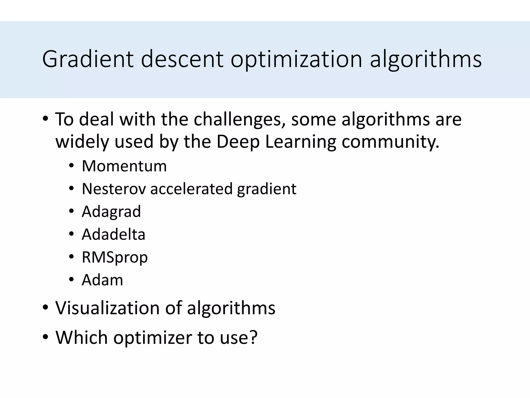
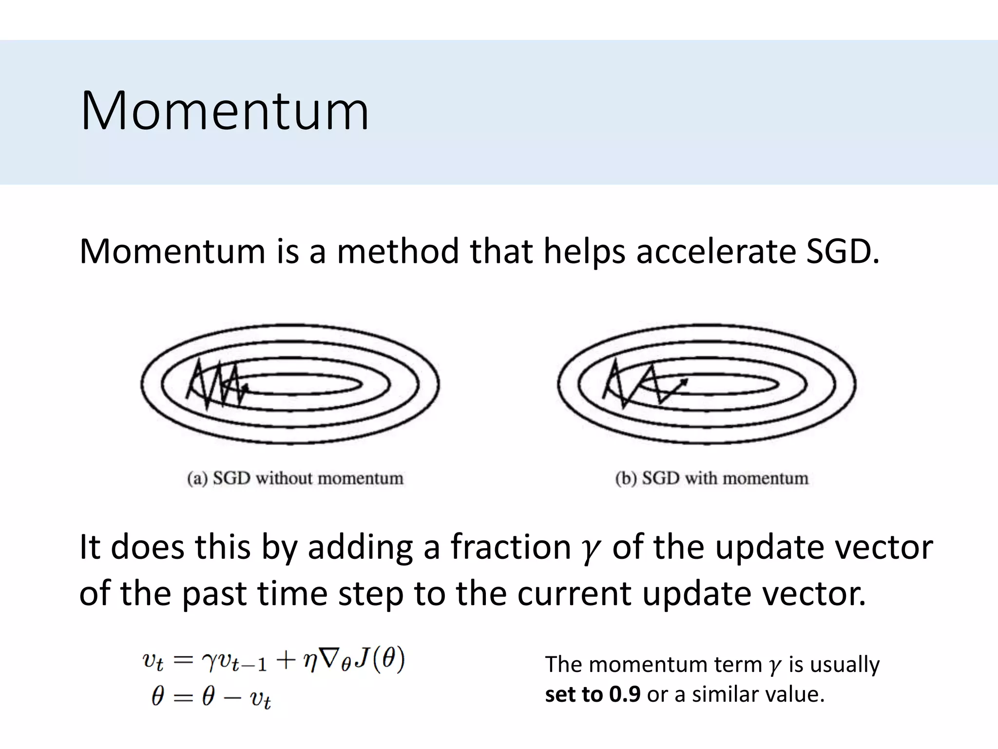
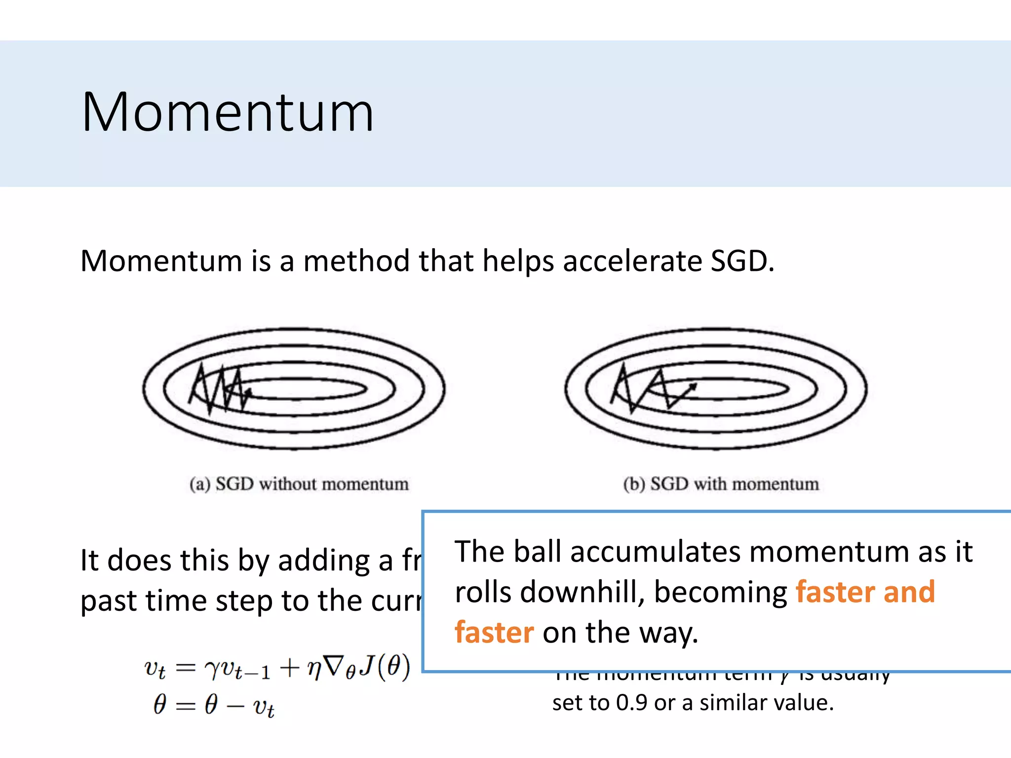
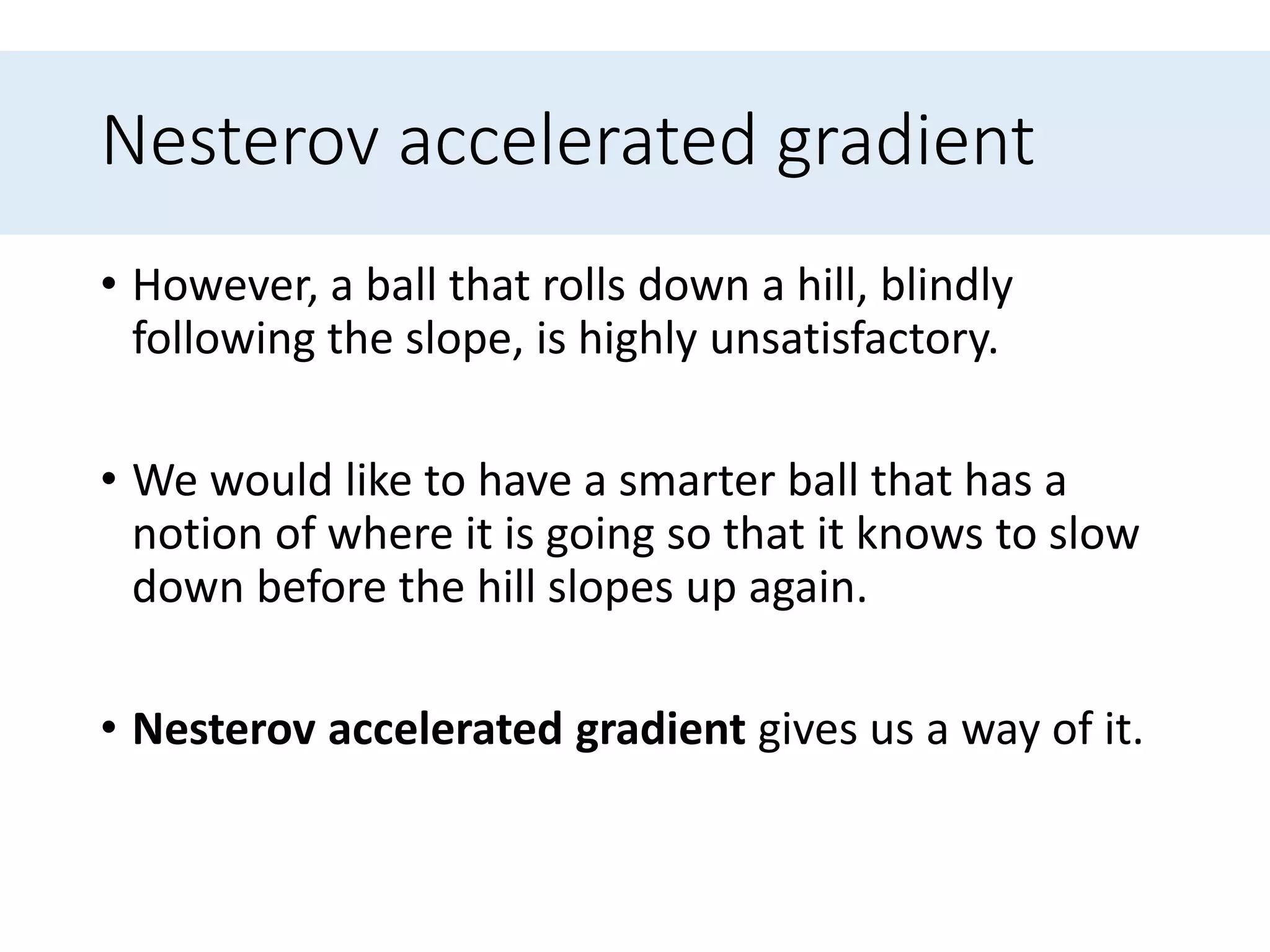
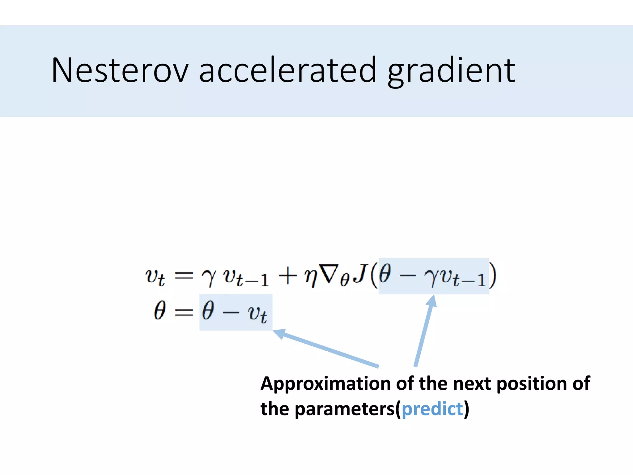
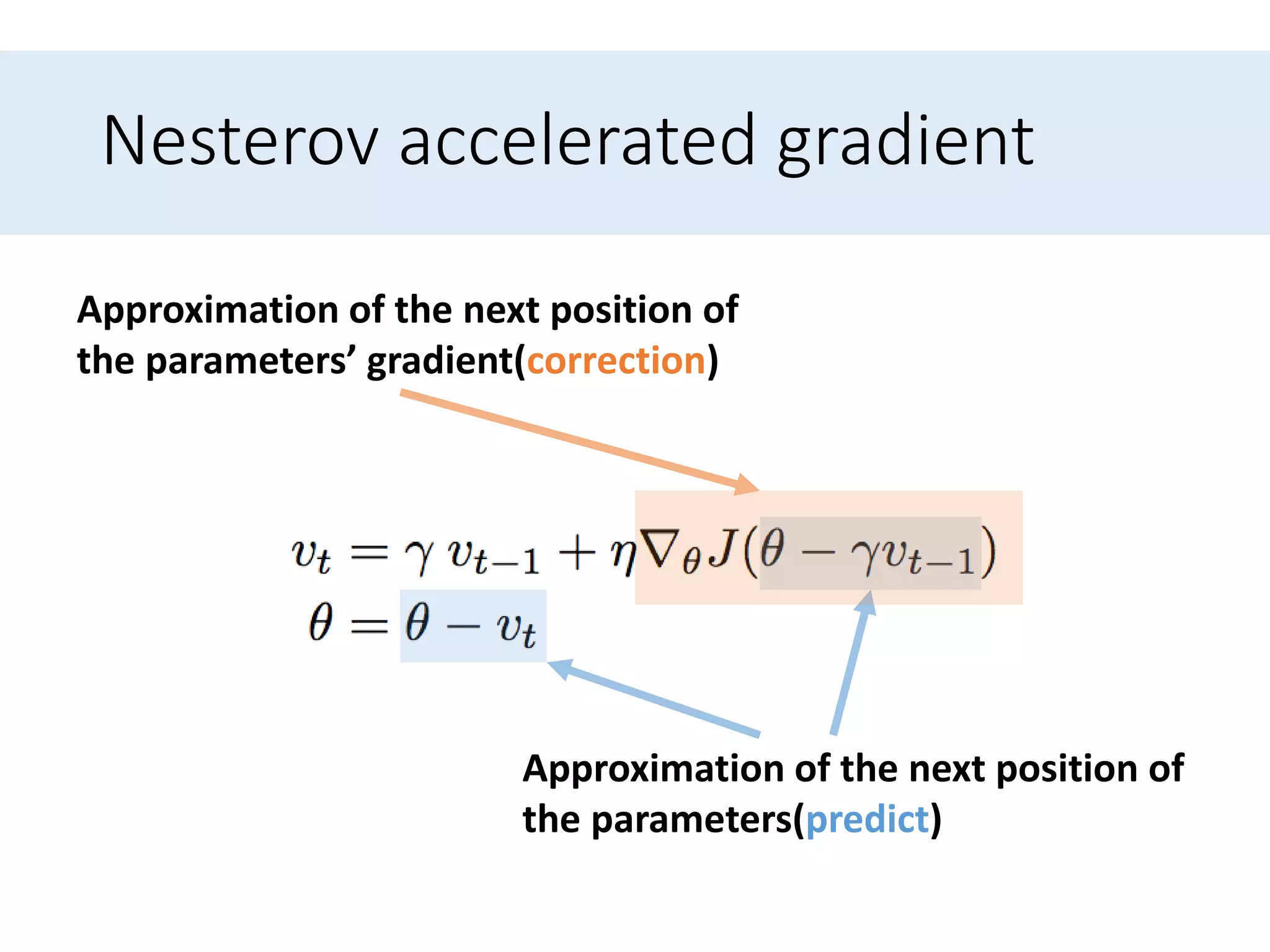
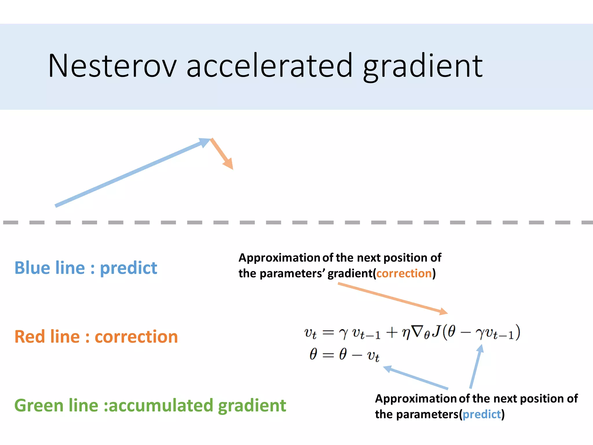
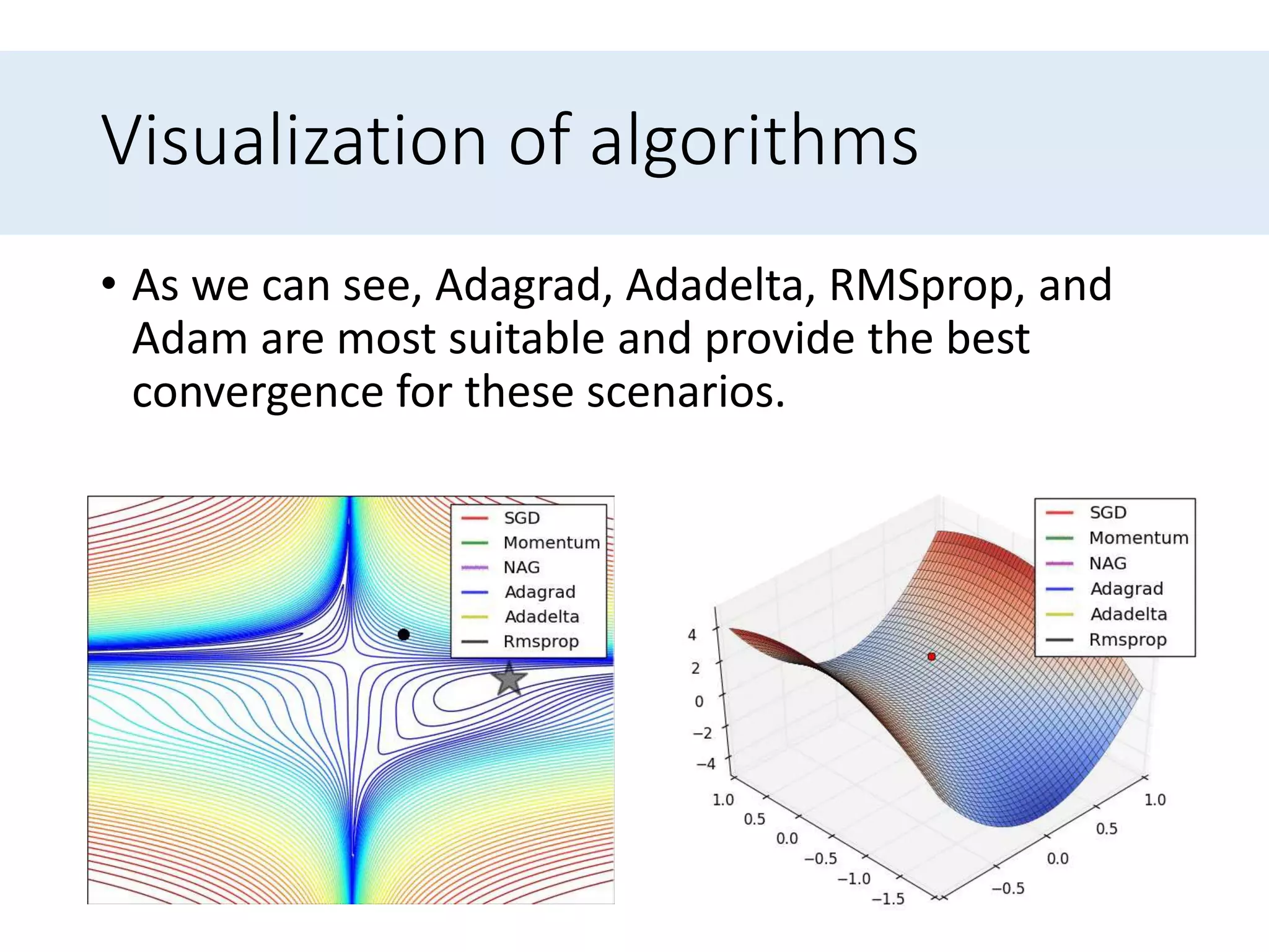
This document provides an overview of various gradient descent optimization algorithms that are commonly used for training deep learning models. It begins with an introduction to gradient descent and its variants, including batch gradient descent, stochastic gradient descent (SGD), and mini-batch gradient descent. It then discusses challenges with these algorithms, such as choosing the learning rate. The document proceeds to explain popular optimization algorithms used to address these challenges, including momentum, Nesterov accelerated gradient, Adagrad, Adadelta, RMSprop, and Adam. It provides visualizations and intuitive explanations of how these algorithms work. Finally, it discusses strategies for parallelizing and optimizing SGD and concludes with a comparison of optimization algorithms.