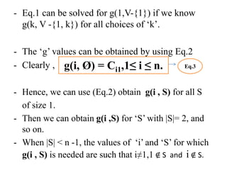
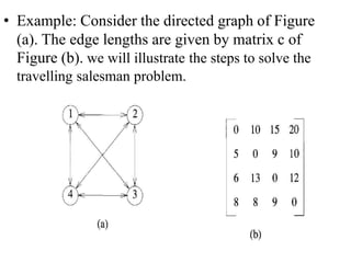
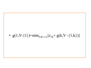
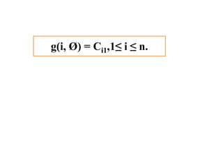
Dynamic programming is used to solve optimization problems by combining solutions to overlapping subproblems. It works by breaking down problems into subproblems, solving each subproblem only once, and storing the solutions in a table to avoid recomputing them. There are two key properties for applying dynamic programming: overlapping subproblems and optimal substructure. Some applications of dynamic programming include finding shortest paths, matrix chain multiplication, the traveling salesperson problem, and knapsack problems.


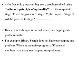


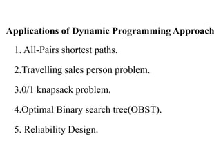


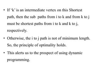
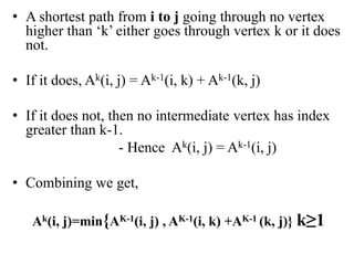


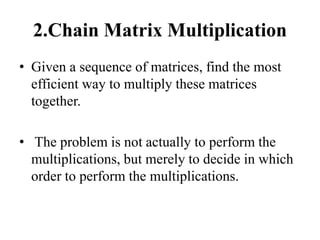
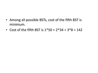
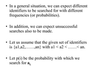
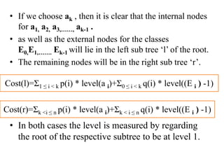
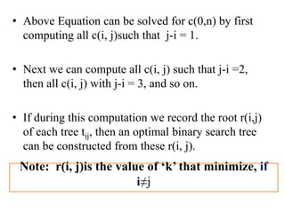
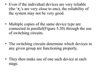
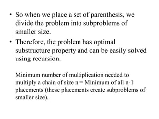
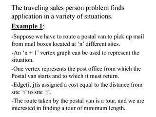
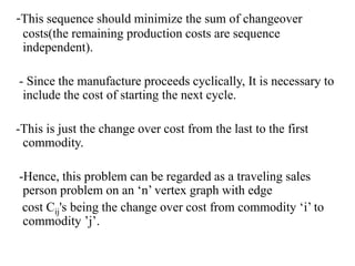
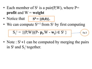
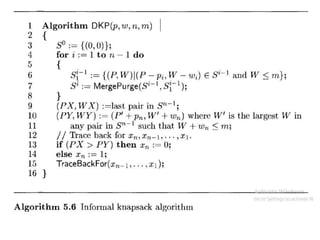
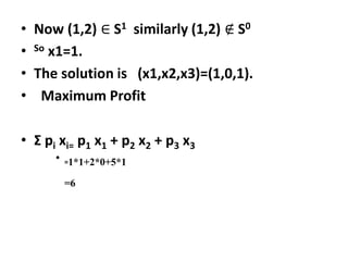
![• Given an array p[] which represents the chain of
matrices such that the ith matrix Ai is of dimension
p[i-1] * p[i].
• We need to write a function MatrixChainOrder() that
should return the minimum number of multiplications
needed to multiply the chain.
• Input: p[] = {40, 20, 30, 10, 30} Output: 26000 There are
4 matrices of dimensions 40x20, 20x30, 30x10 and 10x30.
Let the input 4 matrices be A, B, C and D.
• The minimum number of multiplications are obtained by
putting parenthesis in following way
• (A(BC))D --> 20*30*10 + 40*20*10 + 40*10*30](https://image.slidesharecdn.com/16-210921071310/85/unit-4-dynamic-programming-39-320.jpg)
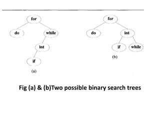
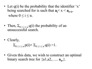
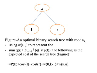
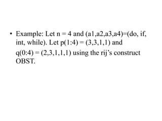
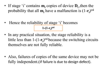
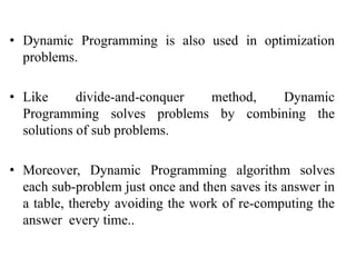
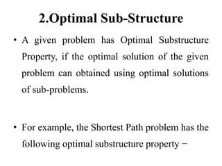
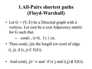
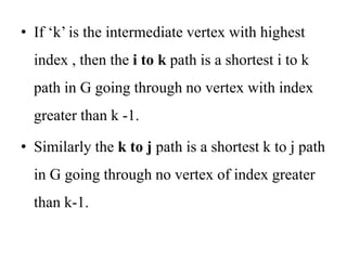
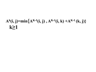
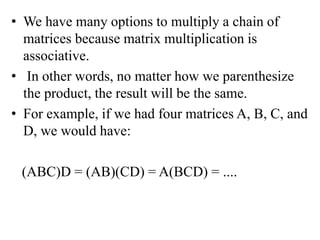
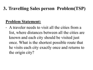
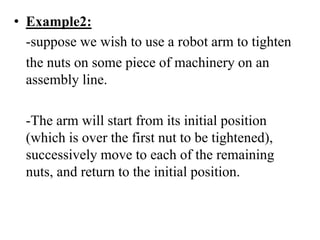
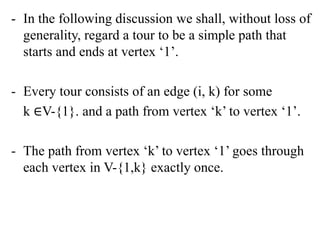
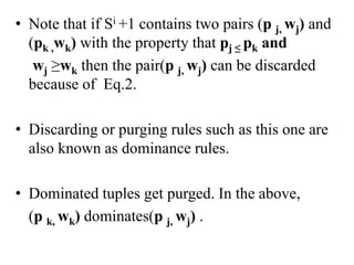
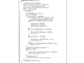
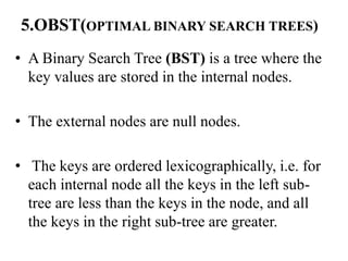
![• Input: p[] = {10, 20, 30, 40, 30} Output: 30000
-There are 4 matrices of dimensions 10x20, 20x30,
30x40 and 40x30.
-Let the input 4 matrices be A, B, C and D. The
minimum number of multiplications are obtained by
putting parenthesis in following way
((AB)C)D --> 10*20*30 + 10*30*40 + 10*40*30
• Input: p[] = {10, 20, 30} Output: 6000
-There are only two matrices of dimensions 10x20 and
20x30.
-So there is only one way to multiply the matrices, cost
of which is 10*20*30](https://image.slidesharecdn.com/16-210921071310/85/unit-4-dynamic-programming-40-320.jpg)
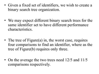
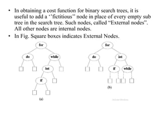
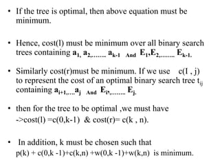
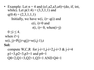
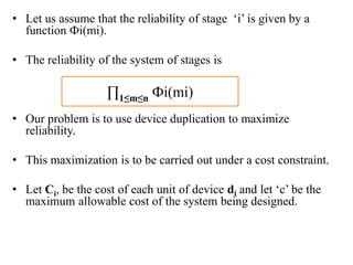
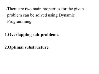
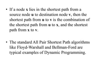
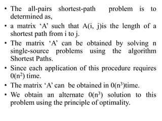
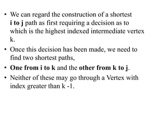
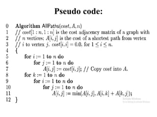
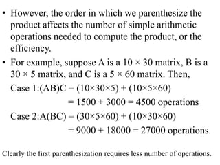
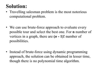
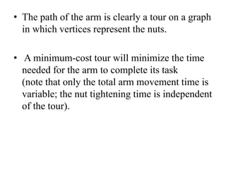
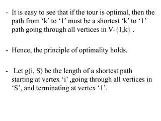
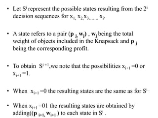
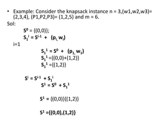
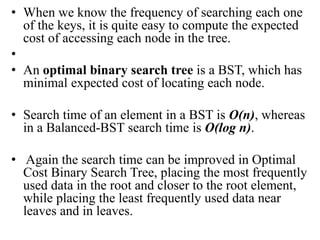
![Pseudocode
Matrix-chain-order (p) ; p =< p1, p2,……….>
1) n ← length[p] − 1
2) for i ← 1 to n
3) do m[i, i] ← 0
4) for l ← 2 to n ; l is length of chain product
5) do for i ← 1 to n − l + 1
6) do j ← i + l −1
7) m[i, j] ← inf
8) for k ← i to j − 1
9) do q ← m[i, k] + m[k+1, j] + pi-1pk pj
10) if q < m[i, j]
11) then m[i, j] ← q
12) s[i, j] ← k
13) return m and s](https://image.slidesharecdn.com/16-210921071310/85/unit-4-dynamic-programming-43-320.jpg)

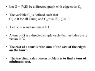
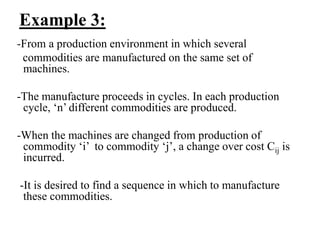
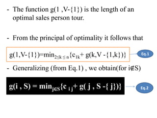


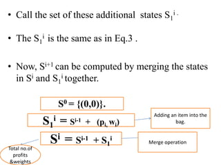


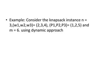


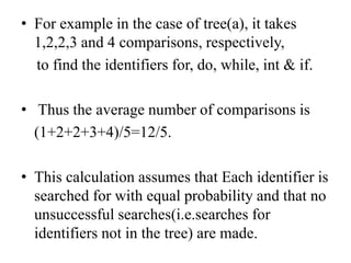
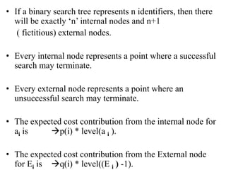
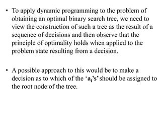
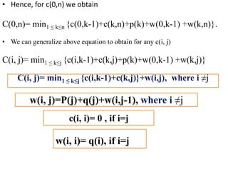
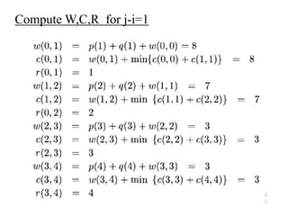
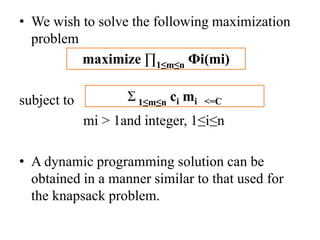
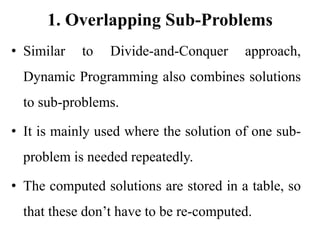
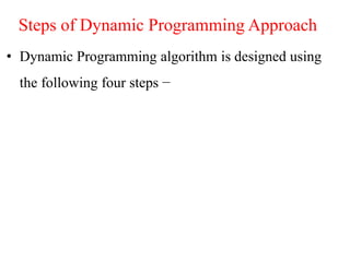
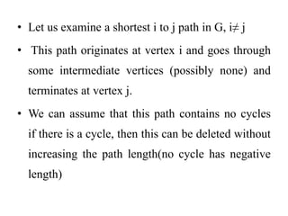
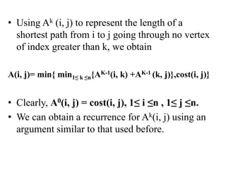
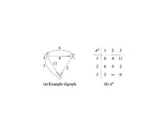
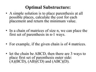
![• Q1.Example: Consider the knapsack instance n
= 5,(w1,w2,w3,w4,w5)= (1,2,5,6,7),
(P1,P2,P3,p4,p5)= (1,6,18,22,28) and m = 11.
Q2.
value = [ 20, 5, 10, 40, 15, 25 ]
weight = [ 1, 2, 3, 8, 7, 4 ]
W = 10](https://image.slidesharecdn.com/16-210921071310/85/unit-4-dynamic-programming-116-320.jpg)


![Input:
value = [ 20, 5, 10, 40, 15, 25 ]
weight = [ 1, 2, 3, 8, 7, 4 ]
W = 10](https://image.slidesharecdn.com/16-210921071310/85/unit-4-dynamic-programming-127-320.jpg)
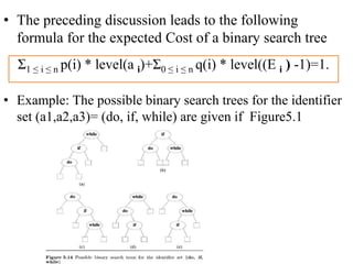
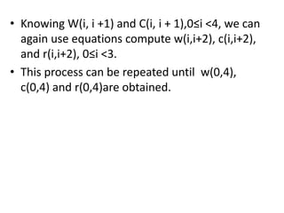
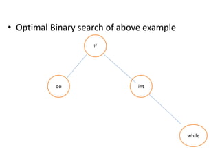
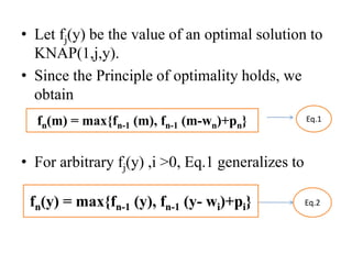
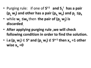
![• Given a sorted array key [0.. n-1] of search keys and an array freq[0.. n-1] of
frequency counts, where freq[i] is the number of searches for keys[i]. Construct a
binary search tree of all keys such that the total cost of all the searches is as small
as possible.
• Let us first define the cost of a BST. The cost of a BST node is the level of that node
multiplied by its frequency. The level of the root is 1.
• Examples:
• Input: keys[] = {10, 12}, freq[] = {34, 50}
• There can be following two possible BSTs
• 10 12
• /
• 12 10
• I II
• Frequency of searches of 10 and 12 are 34 and 50 respectively.
• The cost of tree I is 34*1 + 50*2 = 134
• The cost of tree II is 50*1 + 34*2 = 118](https://image.slidesharecdn.com/16-210921071310/85/unit-4-dynamic-programming-130-320.jpg)
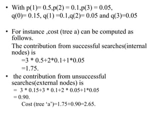
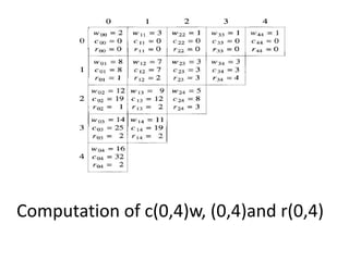
![Given a sorted array key [0.. n-1] of search keys and an array freq[0.. n-1] of
frequency counts, where freq[i] is the number of searches for keys[i]. Construct a
binary search tree of all keys such that the total cost of all the searches is as small
as possible.
Let us first define the cost of a BST. The cost of a BST node is the level of that
node multiplied by its frequency. The level of the root is 1.
Examples:
Input: keys[] = {10, 12}, freq[] = {34, 50}
There can be following two possible BSTs
10 12
/
12 10
I II
Frequency of searches of 10 and 12 are 34 and 50 respectively.
The cost of tree I is 34*1 + 50*2 = 134
The cost of tree II is 50*1 + 34*2 = 118](https://image.slidesharecdn.com/16-210921071310/85/unit-4-dynamic-programming-131-320.jpg)
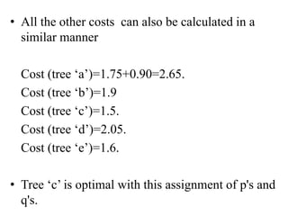
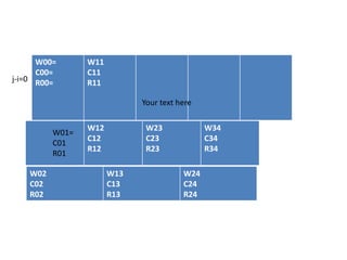
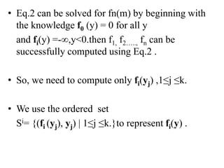
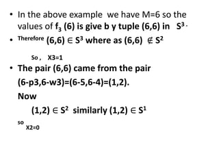
![• Input: keys[] = {10, 12, 20}, freq[] = {34, 8, 50}
• There can be following possible BSTs
• 10 12 20 10 20
• / / /
• 12 10 20 12 20 10
• / /
• 20 10 12 12
• I II III IV V](https://image.slidesharecdn.com/16-210921071310/85/unit-4-dynamic-programming-132-320.jpg)