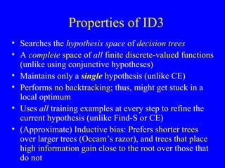
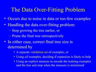
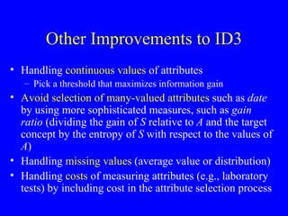
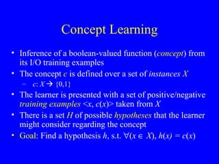
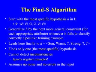
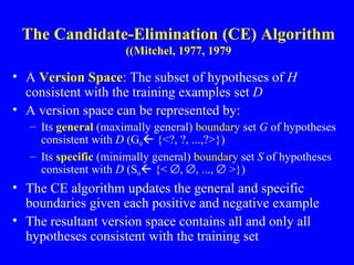
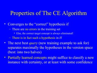
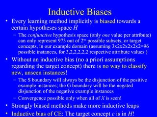
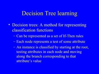
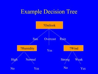
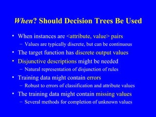
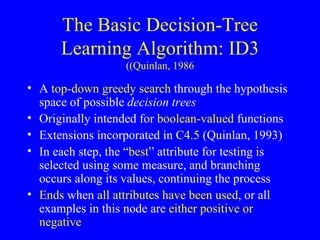
This document discusses machine learning concepts of concept learning and decision-tree learning. It describes concept learning as inferring a boolean function from training examples and using algorithms like Candidate Elimination to search the hypothesis space. Decision tree learning is explained as representing classification functions as trees with nodes testing attributes, allowing disjunctive concepts. The ID3 algorithm is presented as a greedy top-down search that selects the best attribute at each node using information gain, potentially overfitting data without pruning or a validation set.

1. Machine Learning: Concept Learning & Decision-Tree Learning Yuval Shahar M.D., Ph.D. Medical Decision Support Systems

2. Machine Learning Learning: Improving (a program’s) performance in some task with experience Multiple application domains, such as Game playing (e.g., TD-gammon) Speech recognition (e.g., Sphinx) Data mining (e.g., marketing) Driving autonomous vehicles (e.g., ALVINN) Classification of ER and ICU patients Prediction of financial and other fraud Prediction of pneumonia-patients recovery rate

3. Concept Learning Inference of a boolean-valued function ( concept ) from its I/O training examples The concept c is defined over a set of instances X c : X  {0,1} The learner is presented with a set of positive/negative training examples < x , c ( x )> taken from X There is a set H of possible hypotheses that the learner might consider regarding the concept Goal : Find a hypothesis h , s.t.  ( x  X ), h ( x) = c ( x )

4. A Concept-Learning Example Enjoy? Fore-cast Water Wind Humid Air temp Sky # Yes Same Warm Strong Normal Warm Sun 1 Yes Same Warm Strong High Warm Sun 2 No Change Warm Strong High Cold Rain 3 Yes Change Cool Strong High Warm Sun 4

5. The Inductive Learning Hypothesis Any hypothesis approximating the target function well over a large set of training examples will also approximate that target function well over other, unobserved , examples

6. Concept Learning as Search Learning is searching through a large space of hypotheses Space is implicitly defined by the hypothesis representation General-to-specific ordering of hypotheses H1 is more-general-or-equal to H2 if any instance that satisfies H2 also satisfies H1 <Sun, ?, ?, ?, ?, ?>  g <Sun, ?, ?, Strong, ?, ?>

7. The Find-S Algorithm Start with the most specific hypothesis h in H h  <  ,  ,  ,  ,  ,  > Generalize h by the next more general constraint (for each appropriate attribute) whenever it fails to classify correctly a positive training example Leads here finally to h = <Sun, Warm, ?, Strong, ?, ?> Finds only one (the most specific ) hypothesis Cannot detect inconsistencies Ignores negative examples ! Assumes no noise and no errors in the input

8. The Candidate-Elimination (CE) Algorithm (Mitchel, 1977, 1979) A Version Space : The subset of hypotheses of H consistent with the training examples set D A version space can be represented by: Its general (maximally general) boundary set G of hypotheses consistent with D (G 0  {<?, ?, ...,?>}) Its specific (minimally general) boundary set S of hypotheses consistent with D (S 0  {<  ,  , ...,  >}) The CE algorithm updates the general and specific boundaries given each positive and negative example The resultant version space contains all and only all hypotheses consistent with the training set

9. Properties of The CE Algorithm Converges to the “correct” hypothesis if There are no errors in the training set Else, the correct target concept is always eliminated! There is in fact such a hypothesis in H The next best query (new training example to ask for) separates maximally the hypotheses in the version space (best: into two halves) Partially learned concepts might suffice to classify a new instance with certainty, or at least with some confidence

10. Inductive Biases Every learning method implicitly is biased towards a certain hypotheses space H The conjunctive hypothesis space (only one value per attribute) can only represent 973 out of 2 96 possible subsets, or target concepts, in our example domain (assuming 3x2x2x2x2x2=96 possible instances, for 3,2,2,2,2,2 respective attribute values ) Without an inductive bias (no a priori assumptions regarding the target concept) there is no way to classify new, unseen instances ! The S boundary will always be the disjunction of the positive example instances; the G boundary will be the negated disjunction of the negative example instances Convergence possible only when all of X is seen! Strongly biased methods make more inductive leaps Inductive bias of CE : The target concept c is in H !

11. Decision Tree learning Decision trees: A method for representing classification functions Can be represented as a set of If-Then rules Each node represents a test of some attribute An instance is classified by starting at the root, testing attributes in each node and moving along the branch corresponding to that attribute’s value

12. Example Decision Tree Outlook? Humidity? Wind? Yes Yes Yes No No Sun Overcast Rain High Normal Strong Weak

13. When Should Decision Trees Be Used? When instances are <attribute, value> pairs Values are typically discrete, but can be continuous The target function has discrete output values Disjunctive descriptions might be needed Natural representation of disjunction of rules Training data might contain errors Robust to errors of classification and attribute values The training data might contain missing values Several methods for completion of unknown values

14. The Basic Decision-Tree Learning Algorithm: ID3 (Quinlan, 1986) A top-down greedy search through the hypothesis space of possible decision trees Originally intended for boolean-valued functions Extensions incorporated in C4.5 (Quinlan, 1993) In each step, the “ best ” attribute for testing is selected using some measure, and branching occurs along its values, continuing the process Ends when all attributes have been used , or all examples in this node are either positive or negative

15. Which Attribute is Best to Test? The central choice in the ID3 algorithm and similar approaches Here, an information gain measure is used, which measures how well each attribute separates training examples according to their target classification

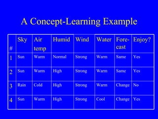
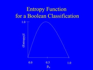
16. Entropy Entropy : An information-theory measure that characterizes the (im)purity of an example set S using the proportion of positive (  ) and negative instances (  ) Informally: Number of bits needed to encode the classification of an arbitrary member of S; Entropy( S ) = –p  log 2 p  – p  log 2 p  Entropy( S ) is in [0..1] Entropy( S ) is 0 if all members are positive or negative Entropy is maximal (1) when p  = p  = 0.5 (uniform distribution of positive and negative cases) If there are c different values to the target concept, Entropy( S ) =  i=1.. c – p i log 2 p i (p i is proportion of class i )

17. Entropy Function for a Boolean Classification p  1.0 0.0 0.5 Entropy( S ) 1.0

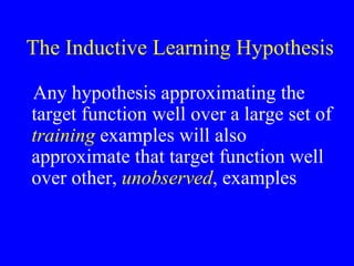
18. Entropy and Surprise Entropy can also be considered as the mean surprise on seeing the outcome (actual class) -log 2 p is also called the surprisal [Tribus, 1961] It is the only nonnegative function consistent with the principle that the amount we are surprised by the occurrence of two independent events with probabilities p 1 and p 2 is the same as we are surprised by the occurrence of a single event with probability p 1 x p 2

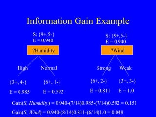
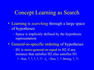
19. Information Gain of an Attribute Sometimes termed the Mutual Information (MI) gained regarding a class (e.g., a disease) given an attribute (e.g., a test), since it is symmetric The expected reduction in entropy E(S) caused by partitioning the examples in S using the attribute A and all its corresponding values Gain( S , A )  E ( S ) –  v  Values( A ) (| S v |/| S |) E (S v ) The attribute with maximal information gain is chosen by ID3 for splitting the node Follows from intuitive axioms [Benish, in press], e.g. not caring how the test result is revealed

20. Information Gain Example Humidity? Wind? {3+, 4-} E = 0.985 High Normal Strong Weak S: {9+,5-} E = 0.940 S: {9+,5-} E = 0.940 {6+, 1-} E = 0.592 {6+, 2-} E = 0.811 {3+, 3-} E = 1.0 Gain( S , Humidity ) = 0.940-(7/14)0.985-(7/14)0.592 = 0.151 Gain( S , Wind ) = 0.940-(8/14)0.811-(6/14)1.0 = 0.048

21. Properties of ID3 Searches the hypothesis space of decision trees A complete space of all finite discrete-valued functions (unlike using conjunctive hypotheses) Maintains only a single hypothesis (unlike CE) Performs no backtracking ; thus, might get stuck in a local optimum Uses all training examples at every step to refine the current hypothesis (unlike Find-S or CE) (Approximate) Inductive bias : Prefers shorter trees over larger trees ( Occam’s razor ), and trees that place high information gain close to the root over those that do not

22. The Data Over-Fitting Problem Occurs due to noise in data or too-few examples Handling the data over-fitting problem: Stop growing the tree earlier, or Prune the final tree retrospectively In either case, correct final tree size is determined by A separate validation set of examples, or Using all examples, deciding if expansion is likely to help Using an explicit measure to encode the training examples and the tree and stop when the measure is minimized

23. Other Improvements to ID3 Handling continuous values of attributes Pick a threshold that maximizes information gain Avoid selection of many-valued attributes such as date by using more sophisticated measures, such as gain ratio (dividing the gain of S relative to A and the target concept by the entropy of S with respect to the values of A ) Handling missing values (average value or distribution) Handling costs of measuring attributes (e.g., laboratory tests) by including cost in the attribute selection process

24. Summary: Concept and Decision-Tree Learning Concept learning is a search through a hypothesis space The Candidate Elimination algorithm uses general-to-specific ordering of hypotheses to compute the version space Inductive learning algorithms can classify unseen examples only because of their implicit inductive bias ID3 searches through the space of decision trees ID3 searches a complete hypothesis space and can handle noise and missing values in the training set Over-fitting the training is a common problem and requires handling by methods such as post-pruning