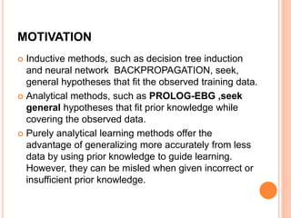
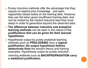
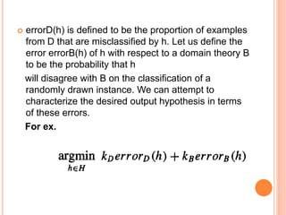
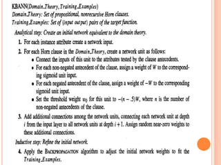
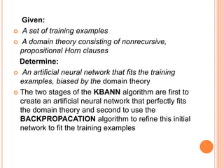
The document discusses combining inductive and analytical learning methods. Inductive methods like decision trees and neural networks seek general hypotheses based solely on training data, while analytical methods like PROLOG-EBG seek hypotheses based on prior knowledge and training data. The document argues that combining these approaches could overcome their individual limitations by using prior knowledge to guide inductive learning methods. It examines using prior knowledge to initialize hypotheses, alter the search objective, and modify the search operators of inductive learners. As an example, it describes the KBANN algorithm, which initializes a neural network to perfectly fit a domain theory before refining it inductively to the training data.

1. COMBINING INDUCTIVE AND
ANALYTICAL LEARNING
SWAPNA.C

2. MOTIVATION
 Inductive methods, such as decision tree induction
and neural network BACKPROPAGATION, seek,
general hypotheses that fit the observed training data.
 Analytical methods, such as PROLOG-EBG ,seek
general hypotheses that fit prior knowledge while
covering the observed data.
 Purely analytical learning methods offer the
advantage of generalizing more accurately from less
data by using prior knowledge to guide learning.
However, they can be misled when given incorrect or
insufficient prior knowledge.

3.  Purely inductive methods offer the advantage that they
require no explicit prior knowledge and learn
regularities based solely on the training data. However,
they can fail when given insufficient training data, and
can be misled by the implicit inductive bias they must
adopt in order to generalize beyond the observed data.
 The difference between inductive and analytical
learning methods can be seen in the nature of the
justifications that can be given for their learned
hypotheses.
 Hypotheses output by purely analytical learning
methods such as PROLOGEBG carry a logical
justification; the output hypothesis follows
deductively from the domain theory and training
examples. Hypotheses output by purely inductive
learning methods such as BACKPROPAGATION carry
a statistical justification;

4.  The output hypothesis follows from statistical arguments
that the training sample is sufficiently large that it is
probably representative of the underlying distribution of
examples. This statistical justification for induction is
clearly articulated in the PAC-learning results.
 Analytical methods provide logically justified hypotheses
and inductive methods provide statistically justified
hypotheses, it is easy to see why
combining them would be useful: Logical Justifications
are only as compelling as the assumptions, or prior
knowledge, on which they are built. They are suspect or
powerless if prior knowledge is incorrect or unavailable.
Statistical justifications are only as compelling as the
data and statistical assumptions on which they rest.

6.  Fig 12.1 summarizes a spectrum of learning
problems that varies by the availability of prior
knowledge and training data. At one extreme, a
large volume of training data is available, but no
prior knowledge. At the other extreme, strong prior
knowledge is available, but little training data. Most
practical learning problems lie somewhere between
these two extremes of the spectrum.
 For example, in analyzing a database of medical
records to learn "symptoms for which treatment x is
more effective than treatment y," one often
begins with approximate prior knowledge (e.g., a
qualitative model of the cause-effect mechanisms
underlying the disease) that suggests the
patient's temperature is more likely to be relevant
than the patient's middle initial.

7.  Similarly, in analyzing a stock market database
to learn the target concept "companies whose stock
value will double over the next 10 months," one
might have approximate knowledge of economic
causes and effects, suggesting that the gross
revenue of the company is more likely to
be relevant than the color of the company logo.
In both of these settings, our own prior knowledge
is incomplete, but is clearly useful in helping
discriminate relevant features from irrelevant.

8.  For example, when applying BACKPROPAGATION to a
problem such as speech recognition, one must choose
the encoding of input and output data, the error function
to be minimized during gradient descent, the number of
hidden units, the topology of the network, the learning
rate and momentum, etc.
 purely inductive instantiation of BACKPROPAGATION,
specialized by the designer's choices to the task of
speech recognition.
 We are interested in systems that take prior knowledge
as an explicit input to the learner, in the same sense
thatthe training data is an explicit input, so that they
remain general purpose algorithms,even while taking
advantage of domain-specific knowledge

9.  Some specific properties we would like from
such a learning method include:
 Given no domain theory, it should learn at least
as effectively as purely inductive methods.
 Given a perfect domain theory, it should learn at
least as effectively as purely analytical methods.
 Given an imperfect domain theory and imperfect
training data, it should combine the two to
outperform either purely inductive or purely
analytical methods.

10.  It should accommodate an unknown level of error in
the training data.
 It should accommodate an unknown level of error
in the domain theory.
 For example, accommodating errors in the training
data is problematic even for statistically based
induction without at least some prior knowledge or
assumption regarding the distribution of errors.
Combining inductive and analytical learning is an
area of active current research.

11. 2 INDUCTIVE-ANALYTICAL APPROACHES TO
LEARNING
2.1 THE LEARNING PROBLEM
Given:
 A set of training examples D, possibly containing
errors
 A domain theory B, possibly containing errors
 A space of candidate hypotheses H
Determine:
 A hypothesis that best fits the training examples and
domain theory

12.  errorD(h) is defined to be the proportion of examples
from D that are misclassified by h. Let us define the
error errorB(h) of h with respect to a domain theory B
to be the probability that h
will disagree with B on the classification of a
randomly drawn instance. We can attempt to
characterize the desired output hypothesis in terms
of these errors.
For ex.

13.  Compute the posterior probability P(h1D) of
hypothesis h given observed training data D. In
particular, Bayes theorem computes this posterior
probability based on the observed data D, together
with prior knowledge in the form of P(h), P(D), and
P(Dlh).
 Thus we can think of P(h), P(D), and P(Dlh) as a form
of background knowledge or domain theory, and we
can think of Bayes theorem as a method for weighting
this domain theory, together with the observed data D,
to assign a posterior probability P(hlD) to h.

14. 2.2 HYPOTHESIS SPACE SEARCH
 One way to understand the range of possible
approaches is to return to our view of learning as a
task of searching through the space of alternative
hypotheses.
 We can characterize most learning methods as
search algorithms by describing the hypothesis
space H they search, the initial hypothesis ho at
which they begin their search, the set of search
operators that define individual search steps, and
the goal criterion G that specifies the search
objective.

15. PRIOR KNOWLEDGE TO ALTER THE SEARCH
PERFORMED BY PURELY INDUCTIVE METHODS.
 Use prior knowledge to derive an initial hypothesis
from which to begin the search.
 In this approach the domain theory B is used to construct
an initial hypothesis ho that is consistent with B. A
standard inductive method
is then applied, starting with the initial hypothesis ho.
Ex. KBANN system prior knowledge to design the
interconnections and weights for an initial network, so that
this initial network is perfectly consistent with the given
domain theory.
 This initial network hypothesis is then refined inductively
using the BACKPROPAGATION algorithm and available
data.

16.  Use prior knowledge to alter the objective of the
hypothesis space search. The goal criterion G is
modified to require that the output hypothesis fits the
domain theory as well as the training examples.
 For example, the EBNN system described below learns
neural networks in this way.
 Whereas inductive learning of neural networks performs
gradient descent search to minimize the squared error of
the network over the training data, EBNN performs
gradient descent to optimize a different criterion.
 Use prior knowledge to alter the available search
steps. In this approach, the set of search operators 0 is
altered by the domain theory. For example, the
 FOCL system described below learns sets of Horn clauses
in this way. It is based on the inductive system FOIL,
which conducts a greedy search through the space of
possible Horn clauses, at each step revising its current
hypothesis by adding a single new literal.

17. 3 USING PRIOR KNOWLEDGE TO
INITIALIZE THE HYPOTHESIS
 One approach to using prior knowledge is to initialize
the hypothesis to perfectly fit the domain theory, then
inductively refine this initial hypothesis as needed to fit
the training data. This approach is used by the KBANN
(Knowledge-Based Artificial Neural Network) algorithm
to learn artificial neural networks.
 In KBANN an initial network is first constructed so that
for every possible instance, the classification assigned
by the network is identical to that assigned by the
domain theory.

18.  If the domain theory is correct, the initial hypothesis
will correctly classify all the training examples and
there will be no need to revise it.
 KBANN is that even if the domain theory is only
approximately correct, initializing the network to fit
this domain theory will give a better starting
approximation to the target function than initializing
the network to random initial weights.
 This initialize-the-hypothesis approach to using
the domain theory has been explored by several
researchers, including Shavlik and Towel1 (1989),
Towel1 and Shavlik (1994), Fu (1989, 1993), and
Pratt (1993a, 1993b).

19. 3.1 THE KBANN ALGORITHM
 The KBANN algorithm exemplifies the initialize-the-
hypothesis approach to using domain theories. It
assumes a domain theory represented by a set of
propositional, nonrecursive Horn clauses.
 A Horn clause is propositional if it contains no
variables. The input and output of KBANN are as
follows:

21. Given:
 A set of training examples
 A domain theory consisting of nonrecursive,
propositional Horn clauses
Determine:
 An artificial neural network that fits the training
examples, biased by the domain theory
 The two stages of the KBANN algorithm are first to
create an artificial neural network that perfectly fits
the domain theory and second to use the
BACKPROPACATION algorithm to refine this initial
network to fit the training examples

22. 3.2 AN ILLUSTRATIVE EXAMPLE
 Adapted from Towel1 and Shavlik (1989). Here
each instance describes a physical object in terms
of the material from which it is made,
whether it is light, etc. The task is to learn the target
concept Cup defined over such physical objects.
The domain theory defines a Cup as an object that
is Stable, Liftable, and an OpenVessel.
 The domain theory also defines each of these
three attributes in terms of more primitive attributes,
tenninating in the primitive, operational attributes
that describe the instances.

23.  KBANN uses the domain theory and training
examples together to learn the target concept more
accurately than it could from either alone.

24.  KBANN uses the domain theory and training examples
together to learn the target concept more accurately
than it could from either alone.
 In the first stage of the KBANN algorithm (steps 1-3 in
the algorithm), an initial network is constructed that is
consistent with the domain theory. For example, the
network constructed from the Cup domain theory is
shown in Figure 12.2.
 In general the network is constructed by creating a
sigmoid threshold unit for each Horn clause in the
domain theory.
 KBANN follows the convention that a sigmoid
output value greater than 0.5 is interpreted as True and
a value below 0.5 as False.
 Each unit is therefore constructed so that its output will
be greater than 0.5 just in those cases where the
corresponding Horn clause applies.

26.  In particular, for each input corresponding to a non-
negated antecedent, the weight is set to some
positive constant W. For each input corresponding
to a negated antecedent, the weight is set to - W.
The threshold weight of the unit, wo is then set to -
(n- .5) W, where n is the number of non-negated
antecedents.
 When unit input values are 1 or 0, this assures that
their weighted sum plus wo will be positive (and
the sigmoid output will therefore be greater than
0.5) if and only if all clause antecedents are
satisfied.
 If a sufficiently large value is chosen for W, this
KBANN algorithm can correctly encode the domain
theory for arbitrarily deep networks.
Towell and Shavlik (1994) report using W = 4.0 in
many of their experiments.

27.  Each sigmoid unit input is connected to the
appropriate network input or to the output of
another sigmoid unit, to mirror the graph of
dependencies among the corresponding attributes
in the domain theory. As a final step many
additional inputs are added to each threshold unit,
with their weights set approximately to
zero.
 The role of these additional connections is to
enable the network to inductively learn additional
dependencies beyond those suggested by the
given domain theory.

28.  The second stage of KBANN (step 4 in the algorithm )
uses the training examples and the
BACKPROPAGATION Algorithm to refine the initial
network weights.
 It is interesting to compare the final, inductively refined
network weights to the initial weights derived from the
domain theory.
 significant new dependencies were discovered during
the inductive step, including the dependency of the
Liftable unit on the feature MadeOfStyrofoam. It is
important to keep in mind that while the unit labeled
Liftable was initially defined by the given Horn clause
for Liftable, the subsequent weight changes performed
by BACKPROPAGATmIOayN h ave dramatically
changed,the meaning of this hiddenunit. After training of
the network, this unit may take on a very different
meaning unrelated to the initial notion of Liftable.

30. 3.3 REMARKS
 KBANN analytically creates a network equivalent to
the given domain theory, then inductively refines
this initial hypothesis to better fit the training data.
In doing so, it modifies the network weights as
needed to overcome inconsistencies between the
domain theory and observed data.
 KBANN generalizes more accurately than
BACKPROPAGATION.