Machine Learning Sections 18.1 - 18.4
What is learning? “ changes in a system that enable a system to do the same task more efficiently the next time” -- Herbert Simon “ constructing or modifying representations of what is being experienced” -- Ryszard Michalski “ making useful changes in our minds” -- Marvin Minsky
Why learn? Understand and improve human learning learn to teach, CAI, CBT Discover new things Data mining Fill in skeletal information about a domain incorporate new information in real time make systems less “finicky” or “brittle” by making them better able to generalize
Components of a learning system
Evaluating Performance Several possible criteria Predictive accuracy of classifier Speed of learner Speed of classifier Space requirements Most common criterion is Predictive Accuracy
Major Paradigms of ML Rote Learning memorize examples Association-based storage and retrieval Induction Learn from examples to reach general conclusions Clustering Analogy Determine correspondence between representations
Major Paradigms (Cont). Discovery Unsupervised, no specific goal Genetic Algorithms Combine successful behaviors, only the fittest survive Reinforcement Feedback (reward) given at end of a sequence of steps Assign rewards by solving a Credit Assignment Problem
Inductive Learning Extrapolate from a given set of examples so that we can make accurate predictions about future examples. Types Supervised teacher tells us the answer y=f(x) Unsupervised predict a future value and then validate Concept Learning Given examples in a class, determine if a test example is in the class (P) or not (N)
Supervised Concept Learning Given a training set of positive and negative examples of a concept construct a description that will accurately classify future examples. Learn some good estimate of function f given a training set: { (x1,y1), (x2,y2), . . . (xn,yn)} where each yi is either + (positive) or - (negative)
Inductive Bias Inductive learning generalizes from specific facts cannot be proven true, but can be proven false Falsity preserving is like searching a Hypothesis Space H of possible f functions Bias allows us to pick which h is preferable define a metric for comparing f functions to find the best
Inductive learning framework Raw input is a feature vector, x, that describes the relevant attributes of an example Each x is a list of n (attribute, value) pairs x = (person=Sue, major=CS, age=Young, Gender=F) Attributes have discrete values.  All examples have all attributes. Each example is a point in n-dimensional feature space
Case-based idea Maintain a library of previous cases When a new problem arises find the most similar case(s) in the library adapt the similar cases to solving the current problem
Nearest Neighbor Save each training example as a point in n-space For each testing example, measure the “distance” to each training example. Classify the example the same as the nearest neighbor Suffers from the curse of high dimensionality Doesn’t generalize well if examples are not clustered tightly
k-nearest neighbor What should the value of k be? That is, how many “close” examples should the algorithm consider? problem dependent Using k nearest neighbors hopefully avoids the problem of noise in the data
Nearest-neighbor problems Storing a large number of examples strategy for deciding whether to keep or discard an example one idea store part of the training data use stored part to predict rest of the training data if mistake, add the mistake to the stored examples Irrelevant features use tuning set to add or remove features to/from the feature set distance function: how much to weight each dimension?
Nearest-neighbor results
Learning Decision Trees Goal: Build a decision tree for classifying examples as positive or negative instances of a concept Supervised Batch processing of training examples using a preference bias
Decision Tree Example
Building Decision Trees Preference Bias is Ockham’s Razor Simplest explanation that is consistent with the observations is probably the best Finding the smallest decision tree is NP-Hard, so we’ll settle for pretty small
Construction Overview Top-down, recursive Pick the “best” attribute for the current node Generate children nodes one for each possible value of the selected attrib Partition the examples on that attribute Assign each subset to the child it goes with repeat for each child until homogeneous
How to pick the “best” attribute? Random Just pick one Least Values narrowest branching of the tree Most Values shallowest tree (fewest levels) Max-Gain largest expected Info Gain smallest expected size of subtrees
Max Gain background Use Information Theory Expected work to guess if an example x in a set S matches a concept: log 2  |S| At each step, we can ask a yes/no question that eliminates at most 1/2 of the elements remaining.
Expected questions remaining Given S = P union N P and N disjoint if x in P, then log 2  |P| questions needed if x in N, then log 2  |N| questions needed (prob(x in P) * log 2  |P|) + (prob(x in N) * log 2  |N|) or, equivalently, (p / (p+n)) * log 2 p + (n / (p+n)) * log 2 n
Information Content How many questions do we save by knowing if x is in P or N? I(P,N) = log 2  |S| - (|P|/|S| log 2  |P|) - (|N|/|S| log 2  |N|) or, equivalently, I(%P, %N) = - (%P log 2 %P) - (%N log 2 %N) Note that 0 <= I(P,N) <= 1, 0 is no info, 1 is max info
Perfect Balance
Example: Homogeneity If all of the samples in S are Positive None are Negative Information content is low
Low Information Content Low information content is desirable in order to make the smallest tree Most of the examples are classified the same The subtree under this node will probably be small
Information Gained For a given attribute measure the difference in Information Content after a node splits up the examples measure the information content at each child weight the information by the proportion of examples that will go there
MaxGain definitions Si = subset of S with value i, i = 1, . . ., m Pi = subset of Si that are + Ni = subset of Si that are - qi = |Si| / |S| = % of examples on branch i %Pi = |Pi| / |Si| = % of + examples on branch i %Ni = |Ni| / |Si| = % of - examples on branch i
Information remaining Weighted sum of information content of each child node generated by that attribute Remainder(A) =     q i  * I(%P i , %N i ) i=1 n
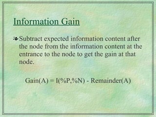
Information Gain Subtract expected information content after the node from the information content at the entrance to the node to get the gain at that node. Gain(A) = I(%P,%N) - Remainder(A)
Select the best attribute Of all the remaining attributes, select the attribute with the highest gain for this location in the decision tree Since entrance information is constant Select A to get the minimum remainder(A)
Example Data
Remainder(Color) 3 of 6 are Red, 2 of 3 are + 3/6 I(2/3, 1/3) = 0.5 * 0.914 = 0.457 1 of 6 are Blue, all are + 1/6 I(1/1, 0/1) = 0.000 2 of 6 are Green, all are - 2/6 I(0/2,2/2) = 0.000 Remainder(Color) = 0.457 + 0.0 + 0.0
Gain Result
Final Decision Tree R B G Big Small
Extensions Real-valued data choose thresholds, each interval becomes a discrete value Noisy data and overfitting 2 examples have identical evidence, but different classifications Some values are inaccurate teacher is wrong Some attributes are irrelevant
Pruning To avoid overfitting choose a threshold for information gain if best remaining attribute is not very good, prune here by making the node a leaf rather than generating children choose a depth limit use a tuning set
Generation of rules For each path from the root to a leaf, translate to a rule: if color=red and size=big then + The collection of rules for all paths from the root to leaves is an interpretation of what the tree means
Setting Parameters Some algorithms require setting learning parameters. Must be set without looking at test data! One method: Tuning Sets Partition data into Train Set and Tune Set For each candidate parameter value, generate decision tree using the Train Set Use Tune set to evaluate error rates and determine which parameter is best Compute new decision tree using selected parameter and entire Training set
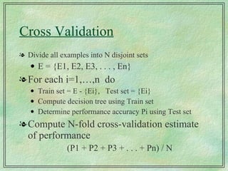
Cross Validation Divide all examples into N disjoint sets E = {E1, E2, E3, . . . , En} For each i=1,…,n  do Train set = E - {Ei},  Test set = {Ei} Compute decision tree using Train set Determine performance accuracy Pi using Test set Compute N-fold cross-validation estimate of performance (P1 + P2 + P3 + . . . + Pn) / N
WillWait from 12 Examples
Increasing Training Set
Summary Decision Trees are widely used Easy to understand rationale Can out-perform humans Fast, simple to implement handles noisy data well Weaknesses Univariate (uses only 1 variable at a time) batch (non-incremental)

Download presentation source

  • 1.
  • 2.
    What is learning?“ changes in a system that enable a system to do the same task more efficiently the next time” -- Herbert Simon “ constructing or modifying representations of what is being experienced” -- Ryszard Michalski “ making useful changes in our minds” -- Marvin Minsky
  • 3.
    Why learn? Understandand improve human learning learn to teach, CAI, CBT Discover new things Data mining Fill in skeletal information about a domain incorporate new information in real time make systems less “finicky” or “brittle” by making them better able to generalize
  • 4.
    Components of alearning system
  • 5.
    Evaluating Performance Severalpossible criteria Predictive accuracy of classifier Speed of learner Speed of classifier Space requirements Most common criterion is Predictive Accuracy
  • 6.
    Major Paradigms ofML Rote Learning memorize examples Association-based storage and retrieval Induction Learn from examples to reach general conclusions Clustering Analogy Determine correspondence between representations
  • 7.
    Major Paradigms (Cont).Discovery Unsupervised, no specific goal Genetic Algorithms Combine successful behaviors, only the fittest survive Reinforcement Feedback (reward) given at end of a sequence of steps Assign rewards by solving a Credit Assignment Problem
  • 8.
    Inductive Learning Extrapolatefrom a given set of examples so that we can make accurate predictions about future examples. Types Supervised teacher tells us the answer y=f(x) Unsupervised predict a future value and then validate Concept Learning Given examples in a class, determine if a test example is in the class (P) or not (N)
  • 9.
    Supervised Concept LearningGiven a training set of positive and negative examples of a concept construct a description that will accurately classify future examples. Learn some good estimate of function f given a training set: { (x1,y1), (x2,y2), . . . (xn,yn)} where each yi is either + (positive) or - (negative)
  • 10.
    Inductive Bias Inductivelearning generalizes from specific facts cannot be proven true, but can be proven false Falsity preserving is like searching a Hypothesis Space H of possible f functions Bias allows us to pick which h is preferable define a metric for comparing f functions to find the best
  • 11.
    Inductive learning frameworkRaw input is a feature vector, x, that describes the relevant attributes of an example Each x is a list of n (attribute, value) pairs x = (person=Sue, major=CS, age=Young, Gender=F) Attributes have discrete values. All examples have all attributes. Each example is a point in n-dimensional feature space
  • 12.
    Case-based idea Maintaina library of previous cases When a new problem arises find the most similar case(s) in the library adapt the similar cases to solving the current problem
  • 13.
    Nearest Neighbor Saveeach training example as a point in n-space For each testing example, measure the “distance” to each training example. Classify the example the same as the nearest neighbor Suffers from the curse of high dimensionality Doesn’t generalize well if examples are not clustered tightly
  • 14.
    k-nearest neighbor Whatshould the value of k be? That is, how many “close” examples should the algorithm consider? problem dependent Using k nearest neighbors hopefully avoids the problem of noise in the data
  • 15.
    Nearest-neighbor problems Storinga large number of examples strategy for deciding whether to keep or discard an example one idea store part of the training data use stored part to predict rest of the training data if mistake, add the mistake to the stored examples Irrelevant features use tuning set to add or remove features to/from the feature set distance function: how much to weight each dimension?
  • 16.
  • 17.
    Learning Decision TreesGoal: Build a decision tree for classifying examples as positive or negative instances of a concept Supervised Batch processing of training examples using a preference bias
  • 18.
  • 19.
    Building Decision TreesPreference Bias is Ockham’s Razor Simplest explanation that is consistent with the observations is probably the best Finding the smallest decision tree is NP-Hard, so we’ll settle for pretty small
  • 20.
    Construction Overview Top-down,recursive Pick the “best” attribute for the current node Generate children nodes one for each possible value of the selected attrib Partition the examples on that attribute Assign each subset to the child it goes with repeat for each child until homogeneous
  • 21.
    How to pickthe “best” attribute? Random Just pick one Least Values narrowest branching of the tree Most Values shallowest tree (fewest levels) Max-Gain largest expected Info Gain smallest expected size of subtrees
  • 22.
    Max Gain backgroundUse Information Theory Expected work to guess if an example x in a set S matches a concept: log 2 |S| At each step, we can ask a yes/no question that eliminates at most 1/2 of the elements remaining.
  • 23.
    Expected questions remainingGiven S = P union N P and N disjoint if x in P, then log 2 |P| questions needed if x in N, then log 2 |N| questions needed (prob(x in P) * log 2 |P|) + (prob(x in N) * log 2 |N|) or, equivalently, (p / (p+n)) * log 2 p + (n / (p+n)) * log 2 n
  • 24.
    Information Content Howmany questions do we save by knowing if x is in P or N? I(P,N) = log 2 |S| - (|P|/|S| log 2 |P|) - (|N|/|S| log 2 |N|) or, equivalently, I(%P, %N) = - (%P log 2 %P) - (%N log 2 %N) Note that 0 <= I(P,N) <= 1, 0 is no info, 1 is max info
  • 25.
  • 26.
    Example: Homogeneity Ifall of the samples in S are Positive None are Negative Information content is low
  • 27.
    Low Information ContentLow information content is desirable in order to make the smallest tree Most of the examples are classified the same The subtree under this node will probably be small
  • 28.
    Information Gained Fora given attribute measure the difference in Information Content after a node splits up the examples measure the information content at each child weight the information by the proportion of examples that will go there
  • 29.
    MaxGain definitions Si= subset of S with value i, i = 1, . . ., m Pi = subset of Si that are + Ni = subset of Si that are - qi = |Si| / |S| = % of examples on branch i %Pi = |Pi| / |Si| = % of + examples on branch i %Ni = |Ni| / |Si| = % of - examples on branch i
  • 30.
    Information remaining Weightedsum of information content of each child node generated by that attribute Remainder(A) =  q i * I(%P i , %N i ) i=1 n
  • 31.
    Information Gain Subtractexpected information content after the node from the information content at the entrance to the node to get the gain at that node. Gain(A) = I(%P,%N) - Remainder(A)
  • 32.
    Select the bestattribute Of all the remaining attributes, select the attribute with the highest gain for this location in the decision tree Since entrance information is constant Select A to get the minimum remainder(A)
  • 33.
  • 34.
    Remainder(Color) 3 of6 are Red, 2 of 3 are + 3/6 I(2/3, 1/3) = 0.5 * 0.914 = 0.457 1 of 6 are Blue, all are + 1/6 I(1/1, 0/1) = 0.000 2 of 6 are Green, all are - 2/6 I(0/2,2/2) = 0.000 Remainder(Color) = 0.457 + 0.0 + 0.0
  • 35.
  • 36.
    Final Decision TreeR B G Big Small
  • 37.
    Extensions Real-valued datachoose thresholds, each interval becomes a discrete value Noisy data and overfitting 2 examples have identical evidence, but different classifications Some values are inaccurate teacher is wrong Some attributes are irrelevant
  • 38.
    Pruning To avoidoverfitting choose a threshold for information gain if best remaining attribute is not very good, prune here by making the node a leaf rather than generating children choose a depth limit use a tuning set
  • 39.
    Generation of rulesFor each path from the root to a leaf, translate to a rule: if color=red and size=big then + The collection of rules for all paths from the root to leaves is an interpretation of what the tree means
  • 40.
    Setting Parameters Somealgorithms require setting learning parameters. Must be set without looking at test data! One method: Tuning Sets Partition data into Train Set and Tune Set For each candidate parameter value, generate decision tree using the Train Set Use Tune set to evaluate error rates and determine which parameter is best Compute new decision tree using selected parameter and entire Training set
  • 41.
    Cross Validation Divideall examples into N disjoint sets E = {E1, E2, E3, . . . , En} For each i=1,…,n do Train set = E - {Ei}, Test set = {Ei} Compute decision tree using Train set Determine performance accuracy Pi using Test set Compute N-fold cross-validation estimate of performance (P1 + P2 + P3 + . . . + Pn) / N
  • 42.
  • 43.
  • 44.
    Summary Decision Treesare widely used Easy to understand rationale Can out-perform humans Fast, simple to implement handles noisy data well Weaknesses Univariate (uses only 1 variable at a time) batch (non-incremental)