Downloaded 11 times


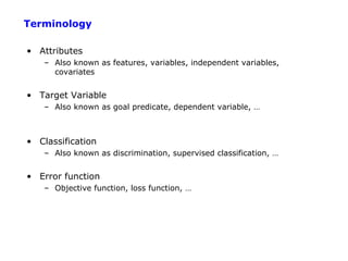
![Empirical Error Functions
• Empirical error function:
E(h) = Σx distance[h(x; θ) , f]
e.g., distance = squared error if h and f are real-valued (regression)
distance = delta-function if h and f are categorical (classification)
Sum is over all training pairs in the training data D
In learning, we get to choose
1. what class of functions h(..) that we want to learn
– potentially a huge space! (“hypothesis space”)
2. what error function/distance to use
- should be chosen to reflect real “loss” in problem
- but often chosen for mathematical/algorithmic convenience](https://image.slidesharecdn.com/machine-learning-120312090810-phpapp01/85/Machine-learning-14-320.jpg)
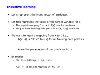
![Inductive Learning as Optimization or Search
• Empirical error function:
E(h) = Σx distance[h(x; θ) , f]
• Empirical learning = finding h(x), or h(x; θ) that minimizes E(h)
• Once we decide on what the functional form of h is, and what the error function E
is, then machine learning typically reduces to a large search or optimization
problem
• Additional aspect: we really want to learn an h(..) that will generalize well to new
data, not just memorize training data – will return to this later](https://image.slidesharecdn.com/machine-learning-120312090810-phpapp01/85/Machine-learning-15-320.jpg)
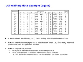

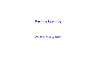
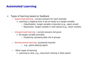
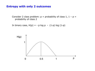
![Entropy
H(p) = entropy of distribution p = {pi}
(called “information” in text)
= E [pi log (1/pi) ] = - p log p - (1-p) log (1-p)
Intuitively log 1/pi is the amount of information we get when we find
out that outcome i occurred, e.g.,
i = “6.0 earthquake in New York today”, p(i) = 1/220
log 1/pi = 20 bits
j = “rained in New York today”, p(i) = ½
log 1/pj = 1 bit
Entropy is the expected amount of information we gain, given a
probability distribution – its our average uncertainty
In general, H(p) is maximized when all pi are equal and minimized
(=0) when one of the pi’s is 1 and all others zero.](https://image.slidesharecdn.com/machine-learning-120312090810-phpapp01/85/Machine-learning-25-320.jpg)
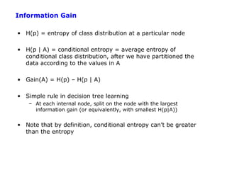
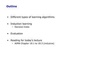
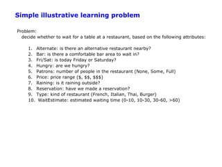
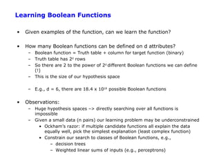
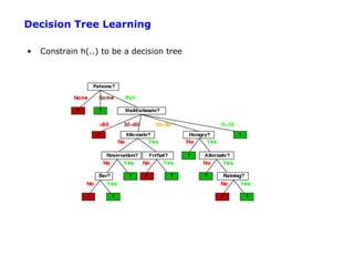
![Root Node Example
For the training set, 6 positives, 6 negatives, H(6/12, 6/12) = 1 bit
Consider the attributes Patrons and Type:
2 4 6 2 4
IG ( Patrons ) = 1 − [ H (0,1) + H (1,0) + H ( , )] = .0541 bits
12 12 12 6 6
2 1 1 2 1 1 4 2 2 4 2 2
IG (Type) = 1 − [ H ( , ) + H ( , ) + H ( , ) + H ( , )] = 0 bits
12 2 2 12 2 2 12 4 4 12 4 4
Patrons has the highest IG of all attributes and so is chosen by the learning
algorithm as the root
Information gain is then repeatedly applied at internal nodes until all leaves contain
only examples from one class or the other](https://image.slidesharecdn.com/machine-learning-120312090810-phpapp01/85/Machine-learning-28-320.jpg)
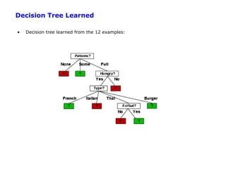
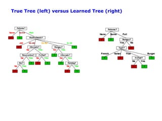

The document discusses machine learning concepts including: 1. Supervised learning aims to learn a function that maps inputs to target variables by minimizing error on training data. Decision tree learning is an example approach. 2. Decision trees partition data into purer subsets using information gain, which measures the reduction in entropy when an attribute is used. 3. The greedy decision tree algorithm recursively selects the attribute with highest information gain to split on, growing subtrees until leaves contain only one class.