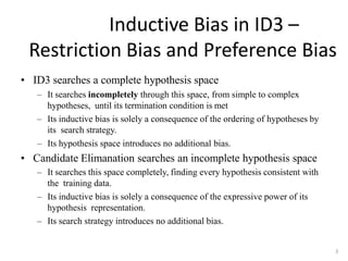
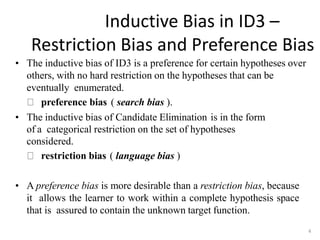
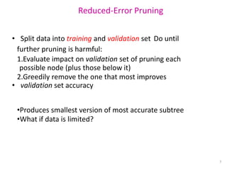
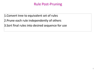
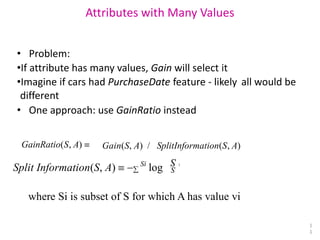
2. 2
Inductive Bias in ID3 -
Occam’s Razor
OCCAM'S RAZOR: Prefer the simplest hypothesis that fits the
data.
Why prefer short hypotheses?
Argument in favor:
– Fewer short hypotheses than long hypotheses
– A short hypothesis that fits the data is unlikely to be a coincidence
– A long hypothesis that fits the data might be a coincidence
Argument opposed:
– There are many ways to define small sets of hypotheses
– What is so special about small sets based on size of hypothesis
3. 3
Inductive Bias in ID3 –
Restriction Bias and Preference Bias
• ID3 searches a complete hypothesis space
– It searches incompletely through this space, from simple to complex
hypotheses, until its termination condition is met
– Its inductive bias is solely a consequence of the ordering of hypotheses by
its search strategy.
– Its hypothesis space introduces no additional bias.
• Candidate Elimanation searches an incomplete hypothesis space
– It searches this space completely, finding every hypothesis consistent with
the training data.
– Its inductive bias is solely a consequence of the expressive power of its
hypothesis representation.
– Its search strategy introduces no additional bias.
4. 4
Inductive Bias in ID3 –
Restriction Bias and Preference Bias
• The inductive bias of ID3 is a preference for certain hypotheses over
others, with no hard restriction on the hypotheses that can be
eventually enumerated.
preference bias ( search bias ).
• The inductive bias of Candidate Elimination is in the form
of a categorical restriction on the set of hypotheses
considered.
restriction bias ( language bias )
• A preference bias is more desirable than a restriction bias, because
it allows the learner to work within a complete hypothesis space
that is assured to contain the unknown target function.
5. Overfitting
• As ID3 adds new nodes to grow the decision tree, the accuracy of the tree
measured over the training examples increases monotonically.
• However, when measured over a set of test examples independent of the
training examples, accuracy first increases, then decreases.
5
6. 6
Avoid Overfitting
How can we avoid overfitting?
– Stop growing when data split not statistically significant
• stop growing the tree earlier, before it reaches the point where it
perfectly classifies the training data
– Grow full tree then post-prune
• allow the tree to overfit the data, and then post-prune the tree.
• The correct tree size is found by stopping early or by post-pruning, a
key question is what criterion is to be used to determine the correct
final tree size.
– Use a separate set of examples, distinct from the training examples, to evaluate
the utility of post-pruning nodes from the tree.
– Use all the available data for training, but apply a statistical test to estimate
whether expanding a particular node is likely to produce an improvement
beyond the training set. ( chi-square test )
7. Reduced-Error Pruning
• Split data into training and validation set Do until
further pruning is harmful:
1.Evaluate impact on validation set of pruning each
possible node (plus those below it)
2.Greedily remove the one that most improves
• validation set accuracy
•Produces smallest version of most accurate subtree
•What if data is limited?
7
8. Rule Post-Pruning
8
1.Convert tree to equivalent set of rules
2.Prune each rule independently of others
3.Sort final rules into desired sequence for use
9. Converting a Tree to Rules
• IF (Type=Car) AND (Doors=2) THEN +
• IF (Type=SUV) AND (Tires=Whitewall) THEN + IF
(Type=Minivan) THEN -
• … (what else?)
9
-
2 4
Doors
Tires
-
2 4
Type
SUV
-
Minivan
+ +
-
4
2 Blackwall
Whitewall
Car
10. Continuous Valued Attributes
• Create one (or more) corresponding discrete attributes
based on continuous
• (EngineSize = 325) = true or false
• (EngineSize <= 330) = t or f (330 is “split” point)
• How to pick best “split” point?
• Sort continuous data
• Look at points where class differs between two values
• Pick the split point with the best gain
1
0
Engine Size: 285 290 295 310 330 330 345 360
Class : - - + + - + + +
11. Attributes with Many Values
• Problem:
•If attribute has many values, Gain will select it
•Imagine if cars had PurchaseDate feature - likely all would be
different
• One approach: use GainRatio instead
1
1
GainRatio(S, A) Gain(S, A) / SplitInformation(S, A)
Split Information(S, A)
Si
log S
i
2
S
where Si is subset of S for which A has value vi
12. Attributes with Costs
• Consider
•medical diagnosis, BloodTest has cost $150
•robotics, Width_from_1ft has cost 23 second
• How to learn consistent tree with low expected cost?
Approaches: replace gain by
• Tan and Schlimmer (1990) Gain2 (S, A) Cost( A)
• Nunez (1988)
• 2Gain( S , A) 1 / (Cost( A) 1)w
• where w [0,1] and determines importance of cost
1
2
13. Unknown Attribute Values
• What if some examples missing values of A?
• “?” in C4.5 data sets
• Use training example anyway, sort through tree
• If node n tests A, assign most common value of A
• among other examples sorted to node n
• assign most common value of A among other examples with same
target value
• assign probability pi to each possible value vi of A
• assign fraction pi of example to each descendant in tree
• Classify new examples in same fashion
1
3
14. 1
4
ASSIGNMENT
1. Explain the inductive biased hypothesis space, unbiased
learner and the futility of Bias Free Learning. Describe the
three types of learner.
2. Describe Inductive Systems and Equivalent Deductive
Systems.
Rank the following three types of leaners according to
their biases:
a. Rote Learner
b. Candidate Elimination Learner
c. Find S Learner.