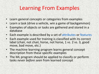
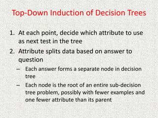
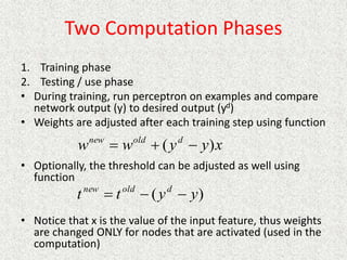
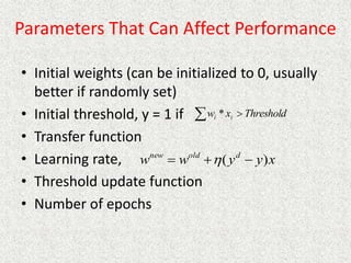
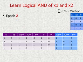
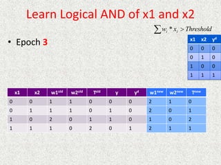
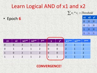
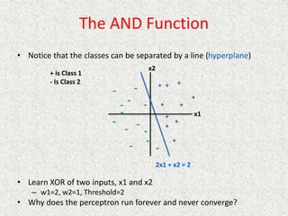
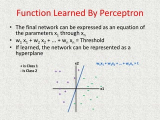
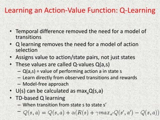
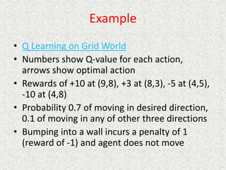
This document discusses machine learning and artificial intelligence concepts such as supervised learning, decision trees, and neural networks. It defines machine learning, describes categories of learning including learning from examples and reinforcement learning, and explains algorithms like naive Bayes classifiers and decision tree induction. Performance measurement and challenges for different machine learning approaches are also summarized.
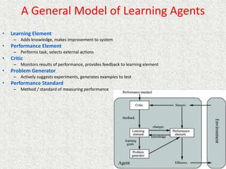
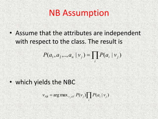


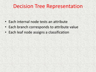
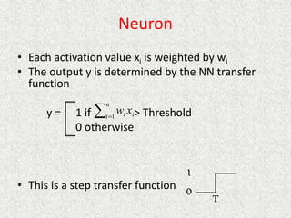


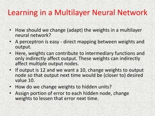

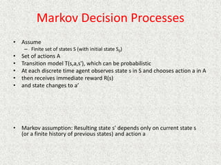
![Passive Learning in a Known Environment
• P(intended move) = 0.8, P(right angles to intended move) = 0.1
• Rewards at terminal states are +1 and -1, other states have reward of -0.04
• From our start position the recommended sequence is [Up, Up, Right,
Right, Right]. This reaches the goal with probability 0.85 = 0.32768.
• Transitions between states are probabilistic, and are represented as a
Markov Decision Process.](https://image.slidesharecdn.com/ai-learningandmachinelearning-230105064600-db9d75b0/85/AI-learning-and-machine-learning-pptx-90-320.jpg)
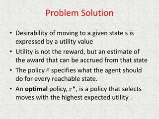
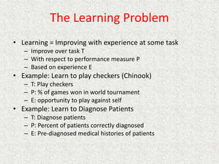
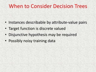
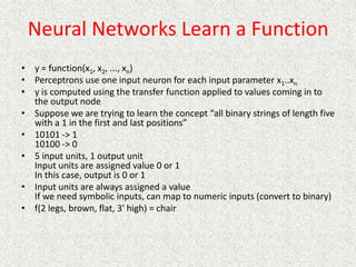
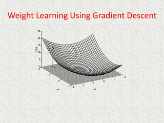
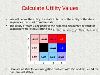
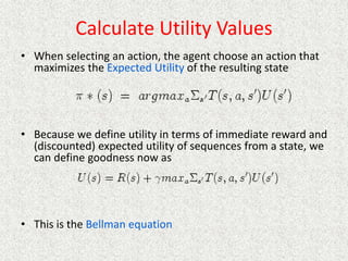
![Define Utility Values
• Learn utilities U of each state, pick action that maximizes expected
utility of resulting state
• Assume infinite horizon
– Agent can move an infinite number of moves in the future
– With fixed horizon of 3, agent would need to head from (3,1) directly to
+1 terminal state
– Given a fixed horizon of N, U([s0, s1, .., sN+k]) = U([s0, s1, .., sN])
• Reward is accumulated over entire sequence of states
– Additive rewards
• Uh[s0, s1, s2, ..] = R(s0) + R(s1) + R(s2) + …
• This could present a problem with infinite horizon problems
– Discounted rewards:
– is a discount factor
– If R is bounded, even for an infinite horizon a discounted reward is finite
– In the limit, R will approach
...
)
(
)
(
)
(
,..]
,
,
[ 2
2
1
0
2
1
0
s
R
s
R
s
R
s
s
s
Uh
1
max
R](https://image.slidesharecdn.com/ai-learningandmachinelearning-230105064600-db9d75b0/85/AI-learning-and-machine-learning-pptx-94-320.jpg)
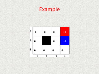
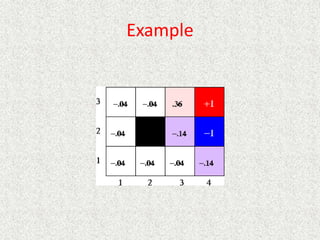
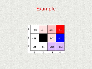
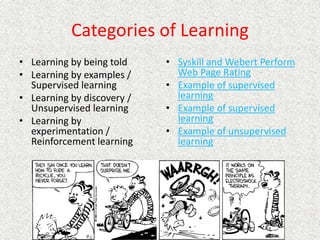
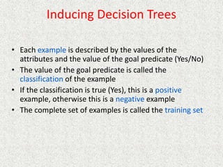
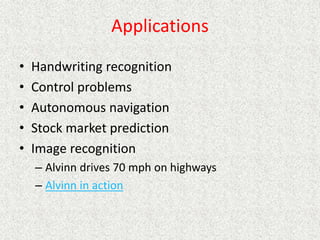
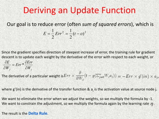
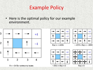
![Example
[RN] shows convergence after 30 iterations](https://image.slidesharecdn.com/ai-learningandmachinelearning-230105064600-db9d75b0/85/AI-learning-and-machine-learning-pptx-101-320.jpg)
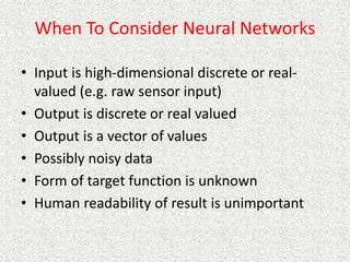
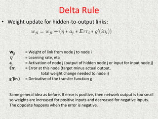
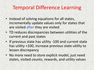
![Adaptive Dynamic Programming
• Learn the transition model
• When a new state is encountered
– Initialize utility to perceived reward for the state
– Keep track of Nsa[s,a] (number of times action a was
executed from state s and Nsas’[s,a,s’] (number of
times action a was executed from state s resulting in
state s’
– T[s,a,s’] = Nsas’[s,a,s’]/Nsa[s,a]
– Update utility as before
• Solve n equations in n unknowns, n = |states|
• Converges slowly](https://image.slidesharecdn.com/ai-learningandmachinelearning-230105064600-db9d75b0/85/AI-learning-and-machine-learning-pptx-103-320.jpg)
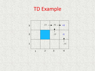
![TD Learning
• Temporal difference (TD)
– When observe transition from state s to state s’
•
• Set U(s') to R(s') the first time s' is visited
• is learning rate
• can decrease as number of visits to s increases
• (N[s])~1/N[s]
• Slower convergence than ADP, but much
simpler with less computation
](https://image.slidesharecdn.com/ai-learningandmachinelearning-230105064600-db9d75b0/85/AI-learning-and-machine-learning-pptx-105-320.jpg)
![Examples
• TD-Gammon [Tesauro, 1995]
– Learn to play Backgammon
– Immediate reward
• +100 if win
• -100 if lose
• 0 for all other states
– Trained by playing 1.5 million games against itself
– Now approximately equal to best human player
• More about TD-Gammon
• Q-Learning applet
• TD Learning applied to Tic Tac Toe
• Move graphic robot across space
• RL applied to channel allocation for cell phones
• RL and robot soccer](https://image.slidesharecdn.com/ai-learningandmachinelearning-230105064600-db9d75b0/85/AI-learning-and-machine-learning-pptx-109-320.jpg)