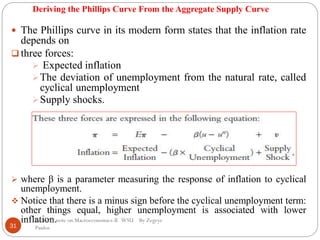
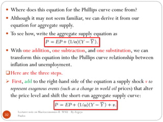
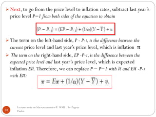
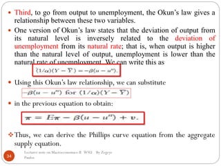
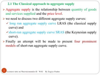
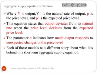
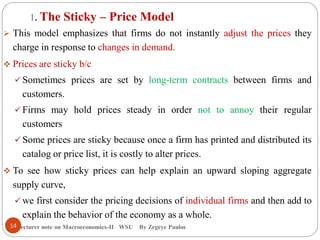
1) The document discusses four models of short-run aggregate supply: the sticky-price model, imperfect information model, and sticky-wage model. 2) In the sticky-price model, some prices are fixed in the short-run due to contracts or costs of changing prices. This can cause output to deviate from natural levels when demand changes. 3) The imperfect information model assumes suppliers don't know the overall price level when making decisions. Output will rise if actual prices are above expected prices. 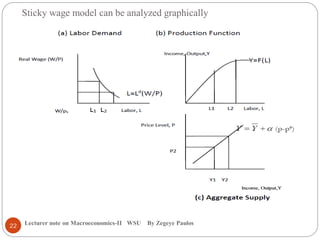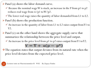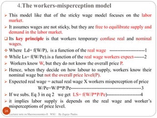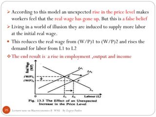4) In the sticky-wage model, nominal wages are fixed by contracts in the short-run. A price rise will lower real wages and induce firms to hire more workers and produce more output

1. CHAPTER TWO
Lecturer note on Macroeconomics-II WSU By Zegeye Paulos
AGGREGATE SUPPLY
1

2. 2.1 The Classical approach to aggregate supply
Lecturer note on Macroeconomics-II WSU By Zegeye Paulos
 Aggregate supply is the relationship between quantity of goods
and services supplied and the price level.
 we need to discuss two different aggregate supply curves:
 long run aggregate supply curve LRAS (the classical supply
curve) and
short-run aggregate supply curve SRAS (the Keynesian supply
curve).
 Finally an attempt will be made to present four prominent
models of short-run aggregate supply curve.
2

3. The Long Run: the Vertical Aggregate Supply Curve
Lecturer note on Macroeconomics-II WSU By Zegeye Paulos
Classical model describes how the economy behaves in
the long run,
we derive the long-run aggregate supply curve from the
classical model.
The classical aggregate supply curve is vertical,
 it is indicating that the same amount of goods will be
supplied whatever the price level or
output does not depend on the price level
 The classical supply curve is based on the assumption
labor market is in equilibrium with full employment
of labor
3

4. Lecturer note on Macroeconomics-II WSU By Zegeye Paulos4

5. Lecturer note on Macroeconomics-II WSU By Zegeye Paulos
If the aggregate supply curve is vertical, then
changes in aggregate demand affect prices but not
output.
For example, if the money supply falls, the
aggregate demand curve shifts downwards.
The economy moves from point A to point B.
If it is an increase in money supply, the
economy moves from A to C.
The shift in aggregate demand affects only prices.
5

6. Lecturer note on Macroeconomics-II WSU By Zegeye Paulos6

7. Lecturer note on Macroeconomics-II WSU By Zegeye Paulos
The classical model and the vertical aggregate supply
curve apply only in the long run.
 In the short run, some prices are sticky and, therefore, do
not adjust to changes in demand.
 Because of this price stickiness, short run aggregate
supply curve is not vertical
This is what we call the Keynesian aggregate supply
curve.
In the extreme Keynesian case
Aggregate supply curve is horizontal;
 Indicating that firms will supply whatever amount of
goods is demanded at the existing price level
7

8. Lecturer note on Macroeconomics-II WSU By Zegeye Paulos8

9. Lecturer note on Macroeconomics-II WSU By Zegeye Paulos
 The idea underlying the Keynesian aggregate supply curve is
that
 because there is unemployment, firms can obtain as much
labor as they want at the current wage.
Their average costs of production therefore are assumed not
to change as their output levels change.
 The short run equilibrium of the economy is obtained
 at the intersection of the AD curve and the horizontal AS
curve.
 In this case changes in aggregate demand either through fiscal
policy or monetary policy
affect the level of out put in the economy.
9

10. Lecturer note on Macroeconomics-II WSU By Zegeye Paulos
Suppose central bank reduces the money supply and
 aggregate demand curve shifts downward .
In the short run, prices are sticky, so the economy
moves from point A to point B.
 Output and employment fall below their natural
levels, which means the economy, is in recession.
Over time, in response to the low demand, wages and
prices fall.
The gradual reduction in the price level moves the
economy down ward along the aggregate demand
curve to pint C, which is the new long run
equilibrium.
10

11. Lecturer note on Macroeconomics-II WSU By Zegeye Paulos11

12. 2.2 The Keynesian approach to aggregate supply
Lecturer note on Macroeconomics-II WSU By Zegeye Paulos
2.2.1 The Four Models of Aggregate Supply
 In the long run, prices are flexible, and the aggregate supply curve
is vertical.
 When the aggregate supply curve is vertical, shifts in the aggregate
demand curve affects the price level, but output remains
unchanged.
 In the short run, prices are sticky, and the aggregate supply curve is not vertical.
 In this case, shifts in the aggregate demand do cause fluctuations in output.
 In extreme Keynesian case where aggregate supply curve is horizontal in which
all prices are fixed.
 In this section we study four models of short-run AS curve.
 Although these models differ in some significant details, but with common
conclusion that short-run aggregate supply curve is upward sloping .
12

13. aggregate supply equation of the form.
Lecturer note on Macroeconomics-II WSU By Zegeye Paulos
Where Y is output, is the natural rate of output, p is
the price level, and pe is the expected price level.
This equation states that output deviates from its natural
rate when the price level deviates from the expected
price level.
The parameter α indicates how much output responds to
unexpected changes in the price level
Each of these models tells different story about what lies
behind this short-run aggregate supply equation.
13

14. 1. The Sticky – Price Model
Lecturer note on Macroeconomics-II WSU By Zegeye Paulos
 This model emphasizes that firms do not instantly adjust the prices they
charge in response to changes in demand.
 Prices are sticky b/c
 Sometimes prices are set by long-term contracts between firms and
customers.
 Firms may hold prices steady in order not to annoy their regular
customers
 Some prices are sticky because once a firm has printed and distributed its
catalog or price list, it is costly to alter prices.
 To see how sticky prices can help explain an upward sloping aggregate
supply curve,
 we first consider the pricing decisions of individual firms and then add to
explain the behavior of the economy as a whole.
14

15. Lecturer note on Macroeconomics-II WSU By Zegeye Paulos
The firm’s desired price P depends
The overall level of prices P &
 The level of aggregate income Y
The overall level of prices P.
 A higher price level implies that the firm’s costs are
higher.
Hence, the higher the overall price level, the more the
firm would like to charge for its product.
The level of aggregate income Y.
 A higher level of income raises the demand for the firm’s
product.
Because marginal cost increases at higher levels of production,
the greater the demand, the higher the firm’s desired price.
)
15

16. We write the firm’s desired pre as
Lecturer note on Macroeconomics-II WSU By Zegeye Paulos
 This equation says that the desired price p depends
on the overall level of prices P and
on the level of aggregate output relative to the natural rate
 The parameter α measures how much the firm’s desired price
responds to the level of aggregate output.
 Now assume that there are two types of firms.
Some have flexible prices: they always set their prices
according to this equation.
Others have sticky prices: they announce their prices in
advance based on what they expect economic conditions to be.
- Firms with sticky prices set prices according to
16
)

17. .
Lecturer note on Macroeconomics-II WSU By Zegeye Paulos
 For simplicity, assume that these firms expect output to be at its
natural rate, so that the last term is zero.
 Then these firms set the price
P= Pe
 We can use the pricing rules of the two groups of firms to derive
the aggregate supply equation.
 To do this, we find the overall price level in the economy, which
is the weighted average of the prices set by the two groups.
 If s is the fraction of firms with sticky prices and
1-s the fraction with flexible-prices,
)
17

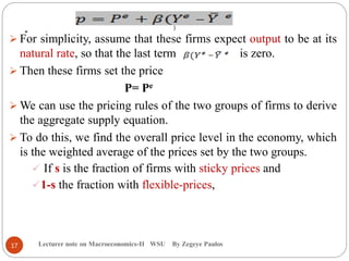
18. Then the overall price level is
Lecturer note on Macroeconomics-II WSU By Zegeye Paulos
 Now subtract (1-s)p from both sides of this equation to obtain
 Divide both sides by s to solve for the overall price level:
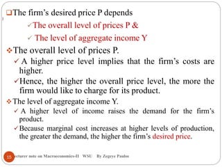
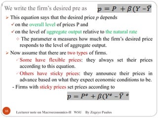
 Hence, the overall all price level depends on the expected price
level and on the level of output.
 where α = s/[1-s) β]. We have
 The deviation of output from the natural rate is positively
associated with the deviation of the price level from the
expected price level.
18

19. 2.The Imperfect Information Model
Lecturer note on Macroeconomics-II WSU By Zegeye Paulos
Assumptions:
 All wages and prices are perfectly flexible, all markets clear.
 Each supplier produces one good, consumes many goods.
 Each supplier knows the nominal price of the good she/he produces, but
does not know the overall price level.
 Supply of each good depends on its relative price: the nominal price of the
good divided by the overall price level.
 Supplier does not know price level at the time he/she makes her production
decision, so uses Pe.
 Suppose P rises but Pe does not.
 Supplier thinks her /his relative price has risen, so she produces more.
 With many producers thinking this way, Y will rise whenever P rises
above Pe
19

20. 3. The Sticky- Wage Model
Lecturer note on Macroeconomics-II WSU By Zegeye Paulos
 In this Model wages are sticky in the short run due to:-
In many industries, nominal wages are set by long-term contracts
Even in industries where there is no such formal contract, implicit
agreements between workers and firms may limit wage changes.
Wages may also depend on social norms and notions of fairness
 To understand the model let us consider what happens to the amount of
output produced when the p rises
When nominal wage is sticky , a rise in the p lowers the real wage
(W/P), making labor cheaper.
The lower real wage induces firms to hire more labor because labor
demand is a function of (W/P).
The additional labor hired produces more output since output(Y) is a
function of employment (L)
20

21. Lecturer note on Macroeconomics-II WSU By Zegeye Paulos
labor demand function L = Ld(W/P)
This function states that the lower the real wage, the more
labor firms hire.
Output is determined by the production function Y=F(L)
This function states that the more labor is hired, the more
output is produced
This positive r/p b/n the price level and the amount of
output means that the aggregate supply curve slopes
upward during the time when nominal wage cannot adjust.
21

22. Sticky wage model can be analyzed graphically
Lecturer note on Macroeconomics-II WSU By Zegeye Paulos22

23. Lecturer note on Macroeconomics-II WSU By Zegeye Paulos
 Panel (a) shows the labor demand curve.
 Because the nominal wageW is stuck, an increase in the P from p1 to p2
reduces real wage from w/p1 toW/p2.
The lower real wage raises the quantity of labor demanded from L1 to L2.
 Panel (b) shows the production function.
 An increase in the quantity of labor from L1 to L2 raises output fromY1 to
Y2.
 Panel (c) on the other hand shows the aggregate supply curve that
summarizes the relationship between the price level and output.
 An increase in the price level from p1 to p2 raises output fromY1 toY2.
The equation states that output deviates from its natural rate when the
price level deviates from the expected price level.
23

24. 4.The workers-misperception model
Lecturer note on Macroeconomics-II WSU By Zegeye Paulos
 This model like that of the sticky wage model focuses on the labor
market.
 It assumes wages are not sticky, but they are free to equilibrate supply and
demand in the labor market.
 Its key principle is that workers temporary confuse real and nominal
wages.
 Where Ld= f(W/P), is a function of the real wage ----------------------1
 While Ls= f(W/Pe).is a function of the real wage workers expect-------2
 Workers know W, but they do not know the overall price P.
 Hence, when they decide on how labour to supply, workers know their
nominal wage but not the overall price level(P).
 Expected real wage = actual real wage X workers misperception of price
W/Pe=W/P*P/Pe--------------------------------------------3
 If we subs. Eq 3 in eq 2 we get LS= f(W/P*P/Pe)---------------------4
 it implies labor supply is depends on the real wage and worker’s
misperceptions of price level.
24

25. Lecturer note on Macroeconomics-II WSU By Zegeye Paulos
 According to this model an unexpected rise in the price level makes
workers feel that the real wage has gone up. But this is a false belief
 Living in a world of illusion they are induced to supply more labor
at the initial real wage.
 This reduces the real wage from (W/P)1 to (W/P)2 and rises the
demand for labor from L1 to L2
The end result is a rise in employment ,output and income
25

26. Conclusion
Lecturer note on Macroeconomics-II WSU By Zegeye Paulos
 In this part we have seen different models of aggregate supply
to explain why the short run aggregate supply curve is
upward sloping.
 Short run equilibrium in the economy can now be explained by
combining aggregate demand and aggregate supply
26

27. Lecturer note on Macroeconomics-II WSU By Zegeye Paulos27

28. Lecturer note on Macroeconomics-II WSU By Zegeye Paulos
 In the short run, the equilibrium moves from point A to B.
 the increase in aggregate demand raises the actual price level from P1
to P2.
 Because people did not expect this increase in the price level, the
expected price level remains at Pe2, and output rises from Y1 to Y2,
which is above the natural rate Y.
 Thus, the unexpected expansion in aggregate demand
 causes the economy to boom.
 Yet the boom does not last forever.
 In the long run, the expected price level rises to catch up with
reality, causing the SR aggregate supply curve to shift upward.
 As the expected price level rises from Pe2 to Pe3, the equilibrium
of the economy moves from point B to point C.
 The actual price level rises from P2 to P3, and output falls from Y2
to Y3 = Y .
 In other words, the economy returns to the natural level of output in
the long run, but at a much higher price level.
28

29. Inflation, Unemployment, and the Phillips Curve
Lecturer note on Macroeconomics-II WSU By Zegeye
Paulos
29
 Two goals of economic policymakers are low inflation and low
unemployment, but often these goals conflict.
 Suppose, for instance, that policymakers were to use monetary
or fiscal policy to expand aggregate demand.
 This policy would move the economy along the short-run
aggregate supply curve to a point of higher output and a higher
price level. (Figure -2 shows this as the change from point A to
point B.)
 Higher output means lower unemployment, because firms
employ more workers when they produce more.
 A higher price level, given the previous year’s price level,
means higher inflation.

30. 30
 Thus, when policymakers move the economy up along the
short-run aggregate supply curve, they reduce the
unemployment rate and raise the inflation rate.
 Conversely, when they contract aggregate demand and move
the economy down the short-run aggregate supply curve,
unemployment rises and inflation falls.
 This tradeoff between inflation and unemployment, called the
Phillips curve
 the Phillips curve is a reflection of the short-run aggregate
supply curve: as policymakers move the economy along the
short-run aggregate supply curve, unemployment and inflation
move in opposite directions.
 The Phillips curve is a useful way to express aggregate supply
because inflation and unemployment are such important
measures of economic performance.Lecturer note on Macroeconomics-II WSU By Zegeye
Paulos

31. Deriving the Phillips Curve From the Aggregate Supply Curve
31
 The Phillips curve in its modern form states that the inflation rate
depends on
 three forces:
 Expected inflation
The deviation of unemployment from the natural rate, called
cyclical unemployment
Supply shocks.
 where β is a parameter measuring the response of inflation to cyclical
unemployment.
 Notice that there is a minus sign before the cyclical unemployment term:
other things equal, higher unemployment is associated with lower
inflation.Lecturer note on Macroeconomics-II WSU By Zegeye
Paulos

32. 32
 Where does this equation for the Phillips curve come from?
 Although it may not seem familiar, we can derive it from our
equation for aggregate supply.
 To see how, write the aggregate supply equation as
 With one addition, one subtraction, and one substitution, we can
transform this equation into the Phillips curve relationship between
inflation and unemployment.
Here are the three steps.
 First, add to the right-hand side of the equation a supply shock v to
represent exogenous events (such as a change in world oil prices) that alter
the price level and shift the short-run aggregate supply curve:
Lecturer note on Macroeconomics-II WSU By Zegeye
Paulos

33. 33
 Next, to go from the price level to inflation rates, subtract last year’s
price level P−1 from both sides of the equation to obtain
 The term on the left-hand side, P - P-1,is the difference between the
current price level and last year’s price level, which is inflation π
 The term on the right-hand side, EP -P-1,is the difference between the
expected price level and last year’s price level, which is expected
inflation Eπ.Therefore, we can replace P − P−1 with π and Eπ -P-1
with Eπ:
Lecturer note on Macroeconomics-II WSU By Zegeye
Paulos

34. 34
 Third, to go from output to unemployment, the Okun’s law gives a
relationship between these two variables.
 One version of Okun’s law states that the deviation of output from
its natural level is inversely related to the deviation of
unemployment from its natural rate; that is, when output is higher
than the natural level of output, unemployment is lower than the
natural rate of unemployment. We can write this as
 Using this Okun’s law relationship, we can substitute
 in the previous equation to obtain:
Thus, we can derive the Phillips curve equation from the aggregate
supply equation.
Lecturer note on Macroeconomics-II WSU By Zegeye
Paulos

35. Lecturer note on Macroeconomics-II WSU By Zegeye Paulos35