- The Phillips curve originally showed an empirical relationship between unemployment and inflation in the UK, but this relationship broke down with sustained inflation. There is actually a trade-off between unemployment and unexpected inflation.
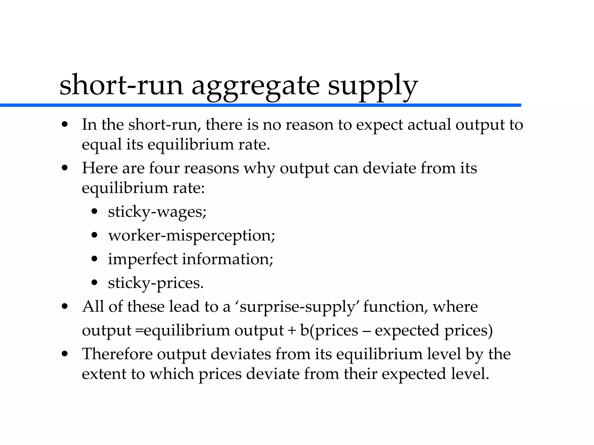
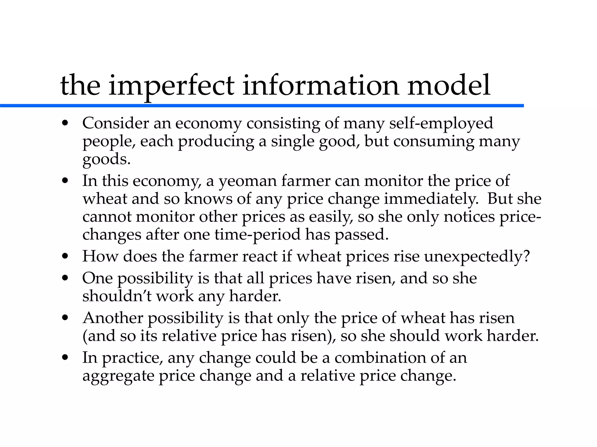
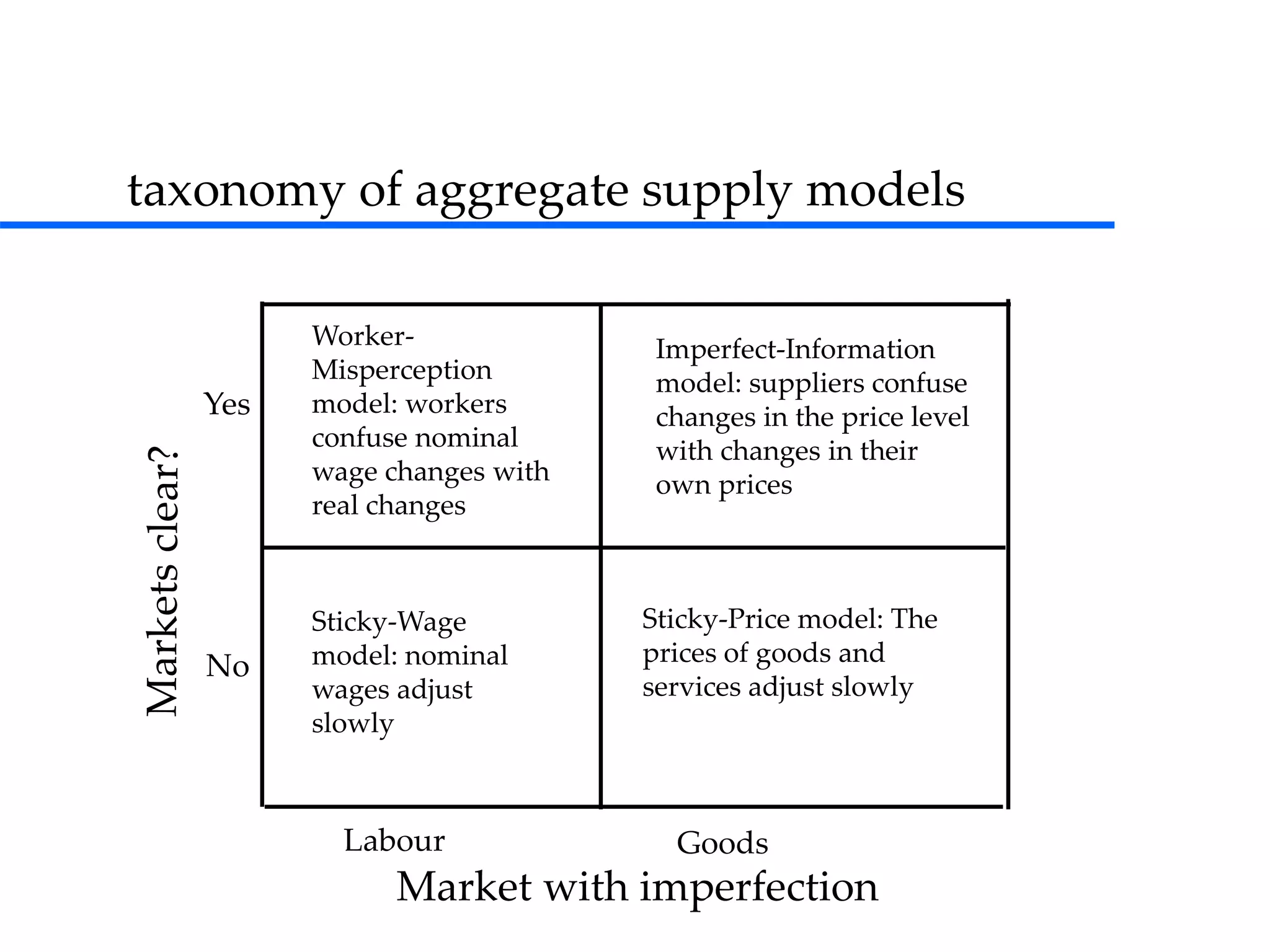
- In the short-run, aggregate supply can deviate from equilibrium output due to sticky wages, worker misperceptions, imperfect information, or sticky prices. This leads to a "surprise supply" function where output depends on the difference between actual and expected prices.
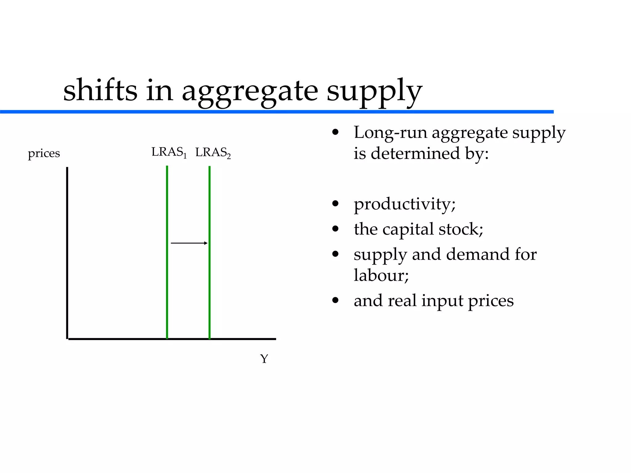
- In the long-run, the natural rate of unemployment and supply-side factors like productivity and input prices determine equilibrium output. Monetary policy influences inflation but not unemployment in the long-run.