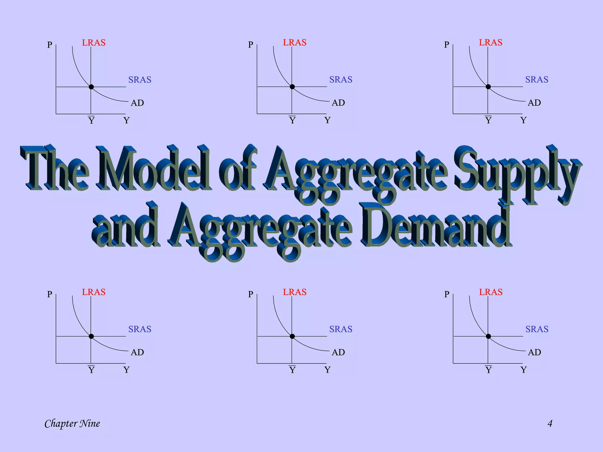
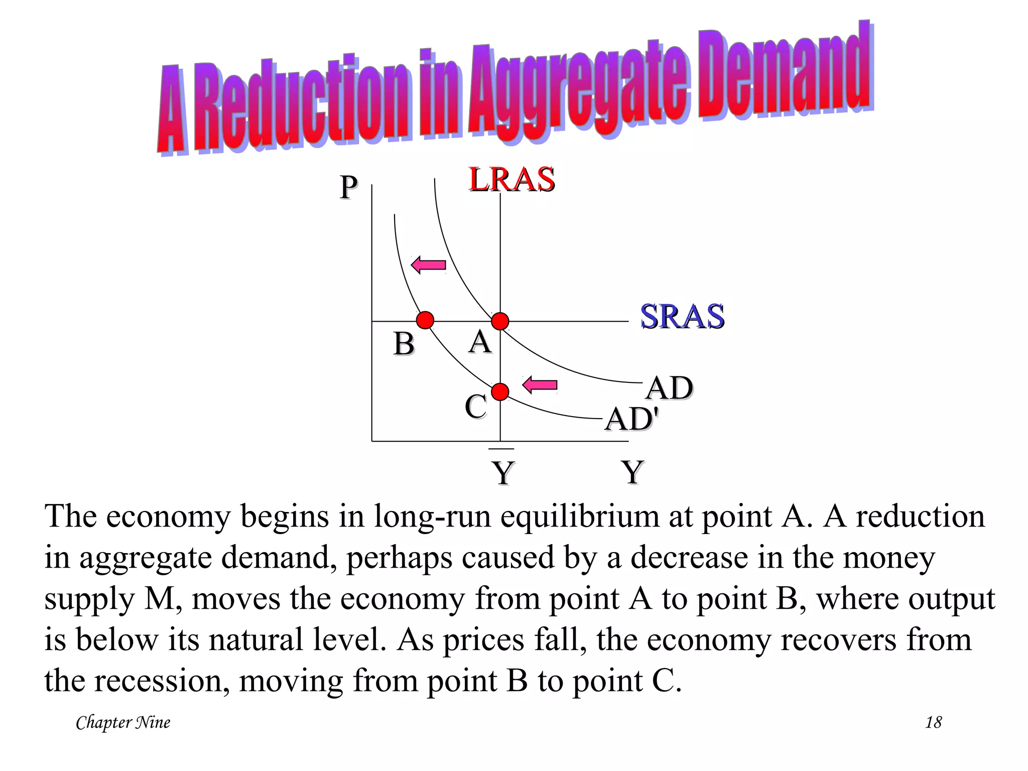
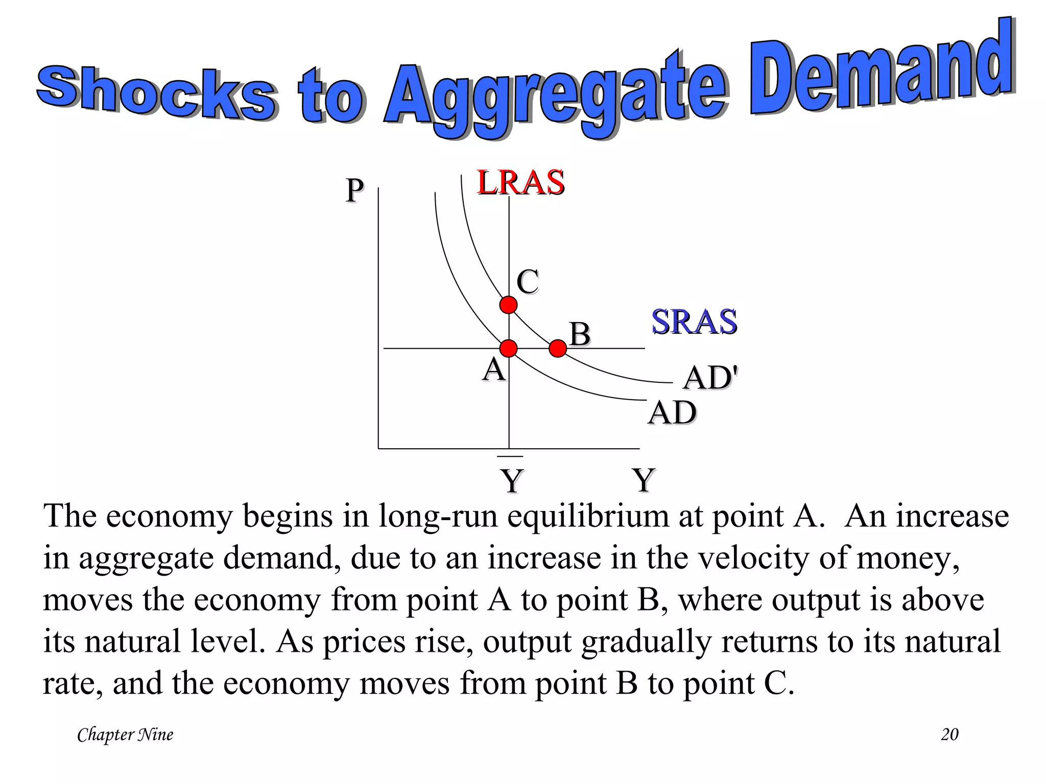
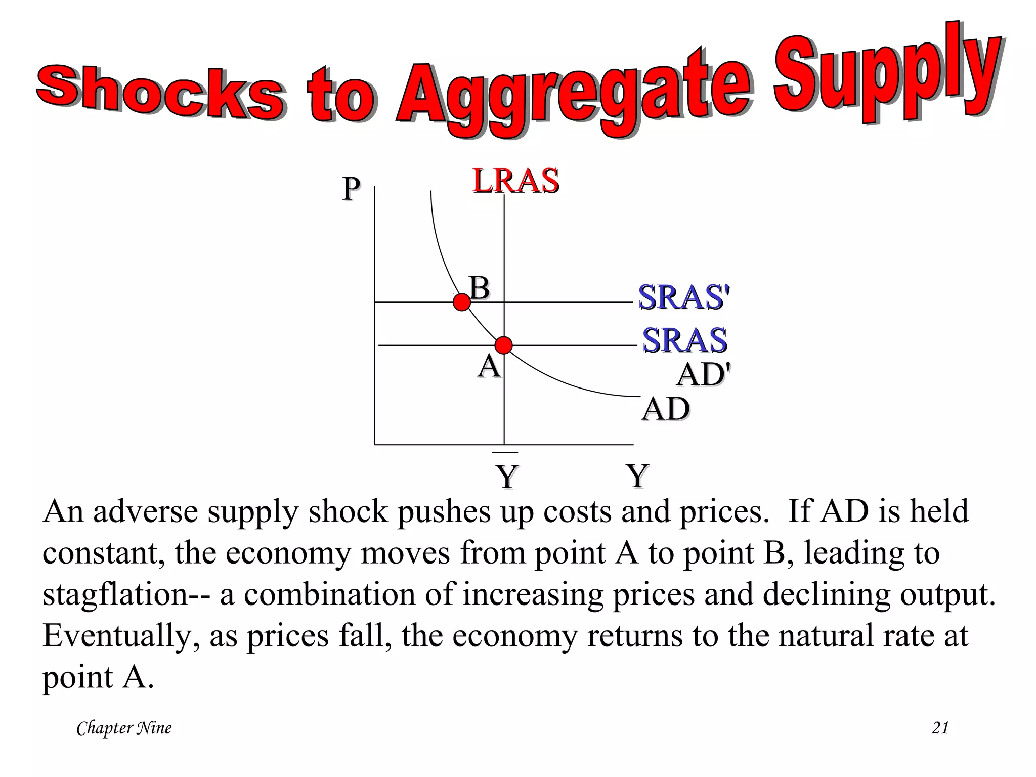
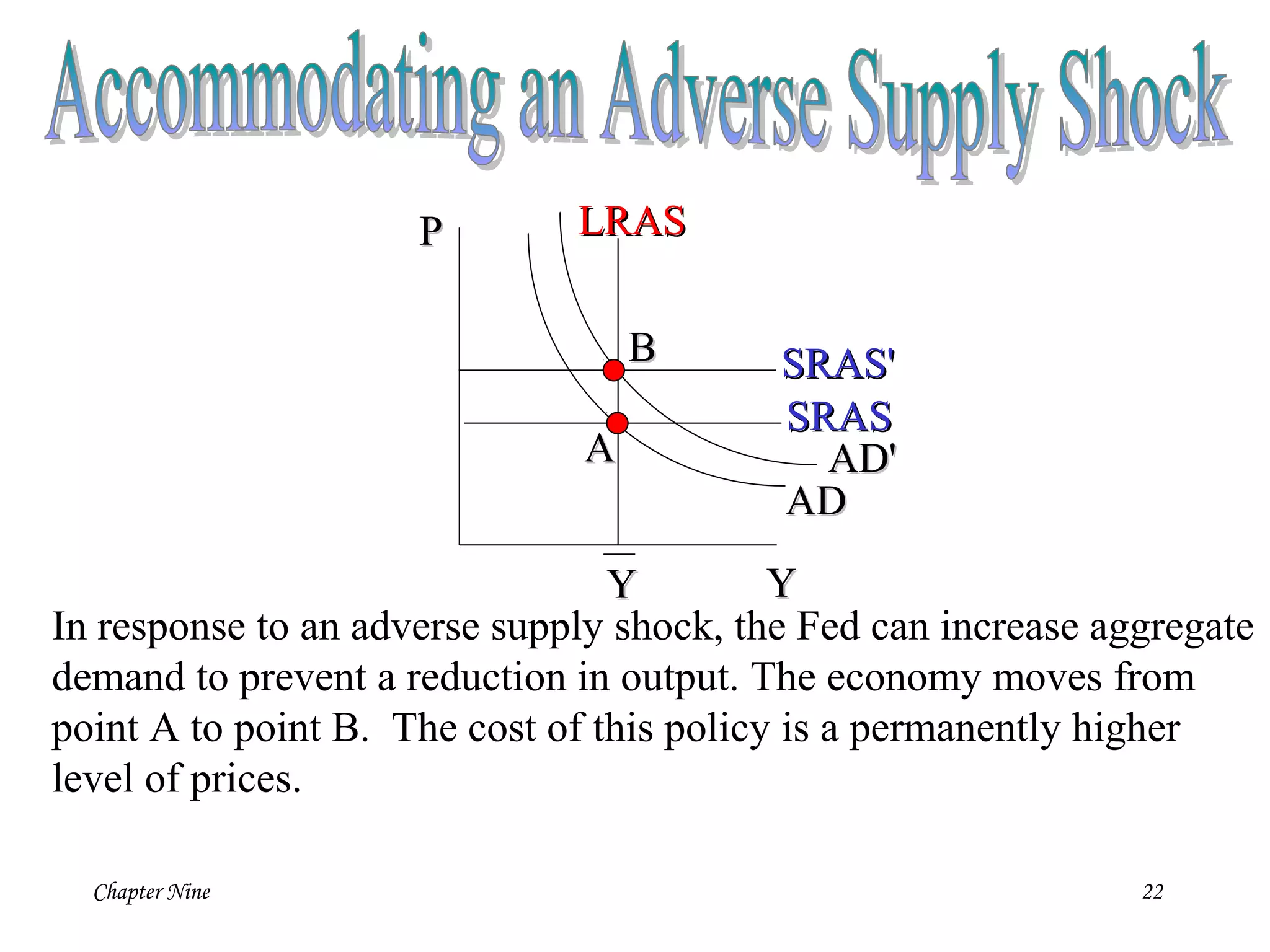
Chapter Nine 1
A PowerPoint™Tutorial
to Accompany macroeconomics, 5th ed.
N. Gregory Mankiw
®
Introduction to Economic Fluctuations
Chapter Nine 2
Short-run fluctuations in output and employment are called the
business cycle. In previous modules, we developed theories to
explain how the economy behaves in the long run.
Those theories were based on the classical dichotomy-- the
premise that real variables, such as output and employment,
are not affected by what happens to nominal variables, such
as the money supply and the price level. Although, the classical
model helps explain long-term trends, most economists agree
that these theories can’t explain short-term
fluctuations in output and employment.
In this module, we will begin to explain these
short-run fluctuations.
Chapter Nine 3
Classical macroeconomic theory applies to the long run but not to
the short run-- WHY?
The short run and long run differ in terms of the treatment of prices.
In the long run, prices are flexible and can respond to changes in
supply or demand. In the short run, many prices are “sticky” at
some predetermined level.
Because prices behave differently in the short run
than in the long run, economic policies have
different effects over different time horizons.
Let’s see this in action.
Chapter Nine 4
PP
YY
LRASLRAS
YY
ADAD
SRASSRAS
PP
YY
LRASLRAS
YY
ADAD
SRASSRAS
PP
YY
LRASLRAS
YY
ADAD
SRASSRAS
PP
YY
LRASLRAS
YY
ADAD
SRASSRAS
PP
YY
LRASLRAS
YY
ADAD
SRASSRAS
PP
YY
LRASLRAS
YY
ADAD
SRASSRAS
PP
YY
LRASLRAS
YY
ADAD
SRASSRAS
PP
YY
LRASLRAS
YY
ADAD
SRASSRAS
PP
YY
LRASLRAS
YY
ADAD
SRASSRAS
PP
YY
LRASLRAS
YY
ADAD
SRASSRAS
PP
YY
LRASLRAS
YY
ADAD
SRASSRAS
PP
YY
LRASLRAS
YY
ADAD
SRASSRAS
Chapter Nine 5
Aggregate demand (AD) is the relationship between the quantity of
output demanded and the aggregate price level. It tells us the quantity
of goods and services people want to buy at any given level of prices.
Recall the Quantity Theory of Money (MV=PY) where M is the money
supply, V is the velocity of money, P is the price level and Y is the
amount of output. It makes the not quite realistic, but very convenient
assumption that velocity is constant over time. Also, recall that the
quantity equation can be rewritten in terms of the supply and demand
for real money balances: M/P = (M/P)d
= kY, where k = 1/V is a
parameter determining how much money people want to hold for every
dollar of income. This equation states that supply of money balances
M/P is equal to the demand and that demand is proportional to output.
Chapter Nine 6
The Aggregate Demand (AD) curve shows the relationship between the
price level P and quantity of goods and services demanded Y. It is
drawn for a given value of the money supply M. The aggregate demand
curve slopes downward: the higher the price level P, the lower the level
of real balances M/P, and therefore the lower the quantity of goods and
services demanded Y.
Pricelevel
Output (Y)
AD
As the price level decreases we’d
move down along the AD curve.
Any changes in M or V would shift
the AD curve.
Remember that the demand for real
output varies inversely with the price
level.
↑Y = MV/↓P
Chapter Nine 7
Think about the supply and demand for real money balances.
If output is higher, people engage in more transactions and
need higher real balances M/P. For a fixed money supply M,
higher real balances imply a lower price level. Conversely, if
the price level is lower, real money balances are higher; the
higher level of real balances allows a greater volume of
transactions,
which means a greater quantity of output is demanded.
Chapter Nine 8
Pricelevel
Output (Y)
AD'
AD
A decrease in the money supply M
reduces the nominal value of output
PY. For any given price level P,
output Y is lower. Thus, a decrease
in the money supply shifts the AD
curve inward from AD to AD'.
A decrease in the money supply M
reduces the nominal value of output
PY. For any given price level P,
output Y is lower. Thus, a decrease
in the money supply shifts the AD
curve inward from AD to AD'.
Chapter Nine 9
Pricelevel
Output (Y)
AD'
AD
An increase in the money supply M
raises the nominal value of output
PY. For any given price level P,
output Y is higher. Thus, an increase
in the money supply shifts the AD
curve outward from AD to AD'.
An increase in the money supply M
raises the nominal value of output
PY. For any given price level P,
output Y is higher. Thus, an increase
in the money supply shifts the AD
curve outward from AD to AD'.
Chapter Nine 10
Aggregate supply (AS) is the relationship
between the quantity of goods and services
supplied and the price level. Because the
firms that supply goods and services have
flexible prices in the long run but sticky
prices in the short run, the aggregate supply
relationship depends on the time horizon.
There are two different aggregate supply curves: the long-run aggregate
supply curve LRAS and the short-run aggregate supply curve (SRAS).
We also must discuss how the economy makes the transition from the
short run to the long run.
But, first, let’s build the long run aggregate supply curve (LRAS).
Chapter Nine 11
Because the classical model describes how the economy behaves in the
long run, we can derive the long-run aggregate supply curve from the
classical model.
Recall the amount of output produced depends on the fixed amounts of
capital and labor and on the available technology.
To show this, we write Y = F(K,L) = Y
According the classical model, output does not depend on the price
level. Let’s think about this considering the market clearing process in
the labor market, the “L” component of the production function.
Chapter Nine 12
Real Wage,
W/PW/P
nndd
Hours Worked
Let’s begin at full employment, n*, with a wage of W/P0.
nn*
W/PW/P00
W/W/22PP00
Now let’s see how workers will respond when there
is a sudden increase in the price level.
nnss
(Employees)
(Employers)
nn′′
At this new lower real wage,
workers will cut back on hours worked.
But, at the same
time, employers
increase their demand
for workers.
nn′′′′ What will happen next?What will happen next?
Chapter Nine 13
W/PW/P
nndd
Hours Worked
nn*
W/W/22PP00
(Employees)
(Employers)
nn′′ nn′′′′
So, right now the labor market is in “disequilibrium” where the quantity
demanded exceeds the quantity supplied.
nnss
We’re now going to see how “flexible wages” will allow the labor
market to come back to equilibrium, at full employment, n*.
To hire more workers, the employer must raise the real wage to 2W.
22W/W/22PP00
As a result of 2W,
more workers are
hired, and the labor market
can move...
Chapter Nine 14
The vertical line suggests that
changes in the price level
will have no lasting impact on
full employment.
The vertical line suggests that
changes in the price level
will have no lasting impact on
full employment.
The mechanism we just went through will enable us
to build our long run aggregate supply curve.
PP
YYYY
Y=F (K,L)
Chapter Nine 15
A reduction in the money
supply shifts the aggregate
demand curve downward
from AD to AD'. Since the
AS curve is vertical in the
long run, the reduction in AD
affects the price level, but not
the level of output.
A reduction in the money
supply shifts the aggregate
demand curve downward
from AD to AD'. Since the
AS curve is vertical in the
long run, the reduction in AD
affects the price level, but not
the level of output.
The vertical aggregate supply curve satisfies the classical dichotomy,
because it implies that the level of output is independent of the money
supply. This long-run level of output, Y is call the full-employment or
natural level of output. It is the level of output at which the economy’s
resources are fully employed, or more realistically, at which
unemployment is at its natural rate.
PP
YYYY
B
A
Chapter Nine 16
Remember that the the vertical LRAS curve assumed that changes in the
price level left no lasting impact on Y (because of the market clearing
process)-- that will be the model for examining the long-term. But we
need a theory for the short-run, defined as the interval of time during
which markets are not fully cleared.
P
Y
LRAS
Y
Y = F (K,L)
P0
AD
AD′A
B
C
A simple, but useful first approach is
to assume short-run price rigidity
meaning that the aggregate supply
curve is flat. As AD shifts to AD′ we
slide in an east-west direction to point
B on the short run aggregate supply
curve (SRAS).
Then, in the long run, we move from
B to C (move up and along AD′).
SRAS
Chapter Nine 17
PP
YY
LRASLRAS
YY
Y = F (K,L)Y = F (K,L)
ADAD
SRASSRAS
In the long run, the economy finds itself at the intersection of the
long-run aggregate supply curve and aggregate demand curve. Because
prices have adjusted to this level, the SRAS crosses this point as well.
Chapter Nine 18
PP
YY
LRASLRAS
YY
ADAD
SRASSRAS
ADAD''
AABB
CC
The economy begins in long-run equilibrium at point A. A reduction
in aggregate demand, perhaps caused by a decrease in the money
supply M, moves the economy from point A to point B, where output
is below its natural level. As prices fall, the economy recovers from
the recession, moving from point B to point C.
Chapter Nine 19
Exogenous changes in aggregate supply or aggregate demand are
called shocks. A shock that affects aggregate supply is called a
supply shock. A shock that affects aggregate demand is called
a demand shock.
A goal of the aggregate demand/aggregate supply model is to help
explain how shocks cause economic fluctuations. Economists use
the term stabilization policy to refer to the policy actions taken to
reduce the severity of short-run economic fluctuations. Stabilization
policy seeks to dampen the business cycle by keeping output and
employment as close to their natural rate as possible.
Chapter Nine 20
PP
YY
LRASLRAS
YY
ADAD
SRASSRAS
ADAD''AA
BB
CC
The economy begins in long-run equilibrium at point A. An increase
in aggregate demand, due to an increase in the velocity of money,
moves the economy from point A to point B, where output is above
its natural level. As prices rise, output gradually returns to its natural
rate, and the economy moves from point B to point C.
Chapter Nine 21
PP
YY
LRASLRAS
YY
ADAD
SRASSRAS
ADAD''AA
BB
An adverse supply shock pushes up costs and prices. If AD is held
constant, the economy moves from point A to point B, leading to
stagflation-- a combination of increasing prices and declining output.
Eventually, as prices fall, the economy returns to the natural rate at
point A.
SRASSRAS''
Chapter Nine 22
PP
YY
LRASLRAS
YY
ADAD
SRASSRAS
ADAD''AA
BB
In response to an adverse supply shock, the Fed can increase aggregate
demand to prevent a reduction in output. The economy moves from
point A to point B. The cost of this policy is a permanently higher
level of prices.
SRASSRAS''
Chapter Nine 23
Aggregate demand
Aggregate supply
Shocks
Demand shocks
Supply shocks
Stabilization policy
Aggregate demand
Aggregate supply
Shocks
Demand shocks
Supply shocks
Stabilization policy

11 1 introduction to economic fluctuations

  • 1.
    Chapter Nine 1 APowerPoint™Tutorial to Accompany macroeconomics, 5th ed. N. Gregory Mankiw ® Introduction to Economic Fluctuations
  • 2.
    Chapter Nine 2 Short-runfluctuations in output and employment are called the business cycle. In previous modules, we developed theories to explain how the economy behaves in the long run. Those theories were based on the classical dichotomy-- the premise that real variables, such as output and employment, are not affected by what happens to nominal variables, such as the money supply and the price level. Although, the classical model helps explain long-term trends, most economists agree that these theories can’t explain short-term fluctuations in output and employment. In this module, we will begin to explain these short-run fluctuations.
  • 3.
    Chapter Nine 3 Classicalmacroeconomic theory applies to the long run but not to the short run-- WHY? The short run and long run differ in terms of the treatment of prices. In the long run, prices are flexible and can respond to changes in supply or demand. In the short run, many prices are “sticky” at some predetermined level. Because prices behave differently in the short run than in the long run, economic policies have different effects over different time horizons. Let’s see this in action.
  • 4.
  • 5.
    Chapter Nine 5 Aggregatedemand (AD) is the relationship between the quantity of output demanded and the aggregate price level. It tells us the quantity of goods and services people want to buy at any given level of prices. Recall the Quantity Theory of Money (MV=PY) where M is the money supply, V is the velocity of money, P is the price level and Y is the amount of output. It makes the not quite realistic, but very convenient assumption that velocity is constant over time. Also, recall that the quantity equation can be rewritten in terms of the supply and demand for real money balances: M/P = (M/P)d = kY, where k = 1/V is a parameter determining how much money people want to hold for every dollar of income. This equation states that supply of money balances M/P is equal to the demand and that demand is proportional to output.
  • 6.
    Chapter Nine 6 TheAggregate Demand (AD) curve shows the relationship between the price level P and quantity of goods and services demanded Y. It is drawn for a given value of the money supply M. The aggregate demand curve slopes downward: the higher the price level P, the lower the level of real balances M/P, and therefore the lower the quantity of goods and services demanded Y. Pricelevel Output (Y) AD As the price level decreases we’d move down along the AD curve. Any changes in M or V would shift the AD curve. Remember that the demand for real output varies inversely with the price level. ↑Y = MV/↓P
  • 7.
    Chapter Nine 7 Thinkabout the supply and demand for real money balances. If output is higher, people engage in more transactions and need higher real balances M/P. For a fixed money supply M, higher real balances imply a lower price level. Conversely, if the price level is lower, real money balances are higher; the higher level of real balances allows a greater volume of transactions, which means a greater quantity of output is demanded.
  • 8.
    Chapter Nine 8 Pricelevel Output(Y) AD' AD A decrease in the money supply M reduces the nominal value of output PY. For any given price level P, output Y is lower. Thus, a decrease in the money supply shifts the AD curve inward from AD to AD'. A decrease in the money supply M reduces the nominal value of output PY. For any given price level P, output Y is lower. Thus, a decrease in the money supply shifts the AD curve inward from AD to AD'.
  • 9.
    Chapter Nine 9 Pricelevel Output(Y) AD' AD An increase in the money supply M raises the nominal value of output PY. For any given price level P, output Y is higher. Thus, an increase in the money supply shifts the AD curve outward from AD to AD'. An increase in the money supply M raises the nominal value of output PY. For any given price level P, output Y is higher. Thus, an increase in the money supply shifts the AD curve outward from AD to AD'.
  • 10.
    Chapter Nine 10 Aggregatesupply (AS) is the relationship between the quantity of goods and services supplied and the price level. Because the firms that supply goods and services have flexible prices in the long run but sticky prices in the short run, the aggregate supply relationship depends on the time horizon. There are two different aggregate supply curves: the long-run aggregate supply curve LRAS and the short-run aggregate supply curve (SRAS). We also must discuss how the economy makes the transition from the short run to the long run. But, first, let’s build the long run aggregate supply curve (LRAS).
  • 11.
    Chapter Nine 11 Becausethe classical model describes how the economy behaves in the long run, we can derive the long-run aggregate supply curve from the classical model. Recall the amount of output produced depends on the fixed amounts of capital and labor and on the available technology. To show this, we write Y = F(K,L) = Y According the classical model, output does not depend on the price level. Let’s think about this considering the market clearing process in the labor market, the “L” component of the production function.
  • 12.
    Chapter Nine 12 RealWage, W/PW/P nndd Hours Worked Let’s begin at full employment, n*, with a wage of W/P0. nn* W/PW/P00 W/W/22PP00 Now let’s see how workers will respond when there is a sudden increase in the price level. nnss (Employees) (Employers) nn′′ At this new lower real wage, workers will cut back on hours worked. But, at the same time, employers increase their demand for workers. nn′′′′ What will happen next?What will happen next?
  • 13.
    Chapter Nine 13 W/PW/P nndd HoursWorked nn* W/W/22PP00 (Employees) (Employers) nn′′ nn′′′′ So, right now the labor market is in “disequilibrium” where the quantity demanded exceeds the quantity supplied. nnss We’re now going to see how “flexible wages” will allow the labor market to come back to equilibrium, at full employment, n*. To hire more workers, the employer must raise the real wage to 2W. 22W/W/22PP00 As a result of 2W, more workers are hired, and the labor market can move...
  • 14.
    Chapter Nine 14 Thevertical line suggests that changes in the price level will have no lasting impact on full employment. The vertical line suggests that changes in the price level will have no lasting impact on full employment. The mechanism we just went through will enable us to build our long run aggregate supply curve. PP YYYY Y=F (K,L)
  • 15.
    Chapter Nine 15 Areduction in the money supply shifts the aggregate demand curve downward from AD to AD'. Since the AS curve is vertical in the long run, the reduction in AD affects the price level, but not the level of output. A reduction in the money supply shifts the aggregate demand curve downward from AD to AD'. Since the AS curve is vertical in the long run, the reduction in AD affects the price level, but not the level of output. The vertical aggregate supply curve satisfies the classical dichotomy, because it implies that the level of output is independent of the money supply. This long-run level of output, Y is call the full-employment or natural level of output. It is the level of output at which the economy’s resources are fully employed, or more realistically, at which unemployment is at its natural rate. PP YYYY B A
  • 16.
    Chapter Nine 16 Rememberthat the the vertical LRAS curve assumed that changes in the price level left no lasting impact on Y (because of the market clearing process)-- that will be the model for examining the long-term. But we need a theory for the short-run, defined as the interval of time during which markets are not fully cleared. P Y LRAS Y Y = F (K,L) P0 AD AD′A B C A simple, but useful first approach is to assume short-run price rigidity meaning that the aggregate supply curve is flat. As AD shifts to AD′ we slide in an east-west direction to point B on the short run aggregate supply curve (SRAS). Then, in the long run, we move from B to C (move up and along AD′). SRAS
  • 17.
    Chapter Nine 17 PP YY LRASLRAS YY Y= F (K,L)Y = F (K,L) ADAD SRASSRAS In the long run, the economy finds itself at the intersection of the long-run aggregate supply curve and aggregate demand curve. Because prices have adjusted to this level, the SRAS crosses this point as well.
  • 18.
    Chapter Nine 18 PP YY LRASLRAS YY ADAD SRASSRAS ADAD'' AABB CC Theeconomy begins in long-run equilibrium at point A. A reduction in aggregate demand, perhaps caused by a decrease in the money supply M, moves the economy from point A to point B, where output is below its natural level. As prices fall, the economy recovers from the recession, moving from point B to point C.
  • 19.
    Chapter Nine 19 Exogenouschanges in aggregate supply or aggregate demand are called shocks. A shock that affects aggregate supply is called a supply shock. A shock that affects aggregate demand is called a demand shock. A goal of the aggregate demand/aggregate supply model is to help explain how shocks cause economic fluctuations. Economists use the term stabilization policy to refer to the policy actions taken to reduce the severity of short-run economic fluctuations. Stabilization policy seeks to dampen the business cycle by keeping output and employment as close to their natural rate as possible.
  • 20.
    Chapter Nine 20 PP YY LRASLRAS YY ADAD SRASSRAS ADAD''AA BB CC Theeconomy begins in long-run equilibrium at point A. An increase in aggregate demand, due to an increase in the velocity of money, moves the economy from point A to point B, where output is above its natural level. As prices rise, output gradually returns to its natural rate, and the economy moves from point B to point C.
  • 21.
    Chapter Nine 21 PP YY LRASLRAS YY ADAD SRASSRAS ADAD''AA BB Anadverse supply shock pushes up costs and prices. If AD is held constant, the economy moves from point A to point B, leading to stagflation-- a combination of increasing prices and declining output. Eventually, as prices fall, the economy returns to the natural rate at point A. SRASSRAS''
  • 22.
    Chapter Nine 22 PP YY LRASLRAS YY ADAD SRASSRAS ADAD''AA BB Inresponse to an adverse supply shock, the Fed can increase aggregate demand to prevent a reduction in output. The economy moves from point A to point B. The cost of this policy is a permanently higher level of prices. SRASSRAS''
  • 23.
    Chapter Nine 23 Aggregatedemand Aggregate supply Shocks Demand shocks Supply shocks Stabilization policy Aggregate demand Aggregate supply Shocks Demand shocks Supply shocks Stabilization policy