Download to read offline


![Solution Continued
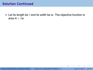
Let its length be ℓ and its width be w. The objective function is
area A = ℓw.
This is a function of two variables, not one. But the perimeter is
fixed.
p − 2w
Since p = 2ℓ + 2w, we have ℓ = , so
2
p − 2w 1 1
A = ℓw = · w = (p − 2w)(w) = pw − w2
2 2 2
Now we have A as a function of w alone (p is constant).
The natural domain of this function is [0, p/2] (we want to make
sure A(w) ≥ 0).
. . . . . .
V63.0121.002.2010Su, Calculus I (NYU) Section 4.5 Optimization Problems June 14, 2010 6 / 31](https://image.slidesharecdn.com/lesson22-optimizationproblemsslides-100615222802-phpapp01-121002230423-phpapp01/85/Lesson22-optimization_problems_slides-14-320.jpg)
![Solution Concluded
1
We use the Closed Interval Method for A(w) = pw − w2 on [0, p/2].
2
At the endpoints, A(0) = A(p/2) = 0.
. . . . . .
V63.0121.002.2010Su, Calculus I (NYU) Section 4.5 Optimization Problems June 14, 2010 7 / 31](https://image.slidesharecdn.com/lesson22-optimizationproblemsslides-100615222802-phpapp01-121002230423-phpapp01/85/Lesson22-optimization_problems_slides-15-320.jpg)
![Solution Concluded
1
We use the Closed Interval Method for A(w) = pw − w2 on [0, p/2].
2
At the endpoints, A(0) = A(p/2) = 0.
dA 1
To find the critical points, we find = p − 2w.
dw 2
. . . . . .
V63.0121.002.2010Su, Calculus I (NYU) Section 4.5 Optimization Problems June 14, 2010 7 / 31](https://image.slidesharecdn.com/lesson22-optimizationproblemsslides-100615222802-phpapp01-121002230423-phpapp01/85/Lesson22-optimization_problems_slides-16-320.jpg)
![Solution Concluded
1
We use the Closed Interval Method for A(w) = pw − w2 on [0, p/2].
2
At the endpoints, A(0) = A(p/2) = 0.
dA 1
To find the critical points, we find = p − 2w.
dw 2
The critical points are when
1 p
0= p − 2w =⇒ w =
2 4
. . . . . .
V63.0121.002.2010Su, Calculus I (NYU) Section 4.5 Optimization Problems June 14, 2010 7 / 31](https://image.slidesharecdn.com/lesson22-optimizationproblemsslides-100615222802-phpapp01-121002230423-phpapp01/85/Lesson22-optimization_problems_slides-17-320.jpg)
![Solution Concluded
1
We use the Closed Interval Method for A(w) = pw − w2 on [0, p/2].
2
At the endpoints, A(0) = A(p/2) = 0.
dA 1
To find the critical points, we find = p − 2w.
dw 2
The critical points are when
1 p
0= p − 2w =⇒ w =
2 4
Since this is the only critical point, it must be the maximum. In this
p
case ℓ = as well.
4
. . . . . .
V63.0121.002.2010Su, Calculus I (NYU) Section 4.5 Optimization Problems June 14, 2010 7 / 31](https://image.slidesharecdn.com/lesson22-optimizationproblemsslides-100615222802-phpapp01-121002230423-phpapp01/85/Lesson22-optimization_problems_slides-18-320.jpg)
![Solution Concluded
1
We use the Closed Interval Method for A(w) = pw − w2 on [0, p/2].
2
At the endpoints, A(0) = A(p/2) = 0.
dA 1
To find the critical points, we find = p − 2w.
dw 2
The critical points are when
1 p
0= p − 2w =⇒ w =
2 4
Since this is the only critical point, it must be the maximum. In this
p
case ℓ = as well.
4
We have a square! The maximal area is A(p/4) = p2 /16.
. . . . . .
V63.0121.002.2010Su, Calculus I (NYU) Section 4.5 Optimization Problems June 14, 2010 7 / 31](https://image.slidesharecdn.com/lesson22-optimizationproblemsslides-100615222802-phpapp01-121002230423-phpapp01/85/Lesson22-optimization_problems_slides-19-320.jpg)


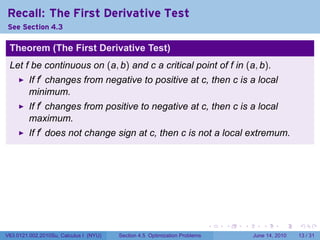
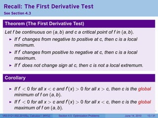
![Recall: The Closed Interval Method
See Section 4.1
The Closed Interval Method
To find the extreme values of a function f on [a, b], we need to:
Evaluate f at the endpoints a and b
Evaluate f at the critical points x where either f′ (x) = 0 or f is not
differentiable at x.
The points with the largest function value are the global maximum
points
The points with the smallest/most negative function value are the
global minimum points.
. . . . . .
V63.0121.002.2010Su, Calculus I (NYU) Section 4.5 Optimization Problems June 14, 2010 12 / 31](https://image.slidesharecdn.com/lesson22-optimizationproblemsslides-100615222802-phpapp01-121002230423-phpapp01/85/Lesson22-optimization_problems_slides-29-320.jpg)
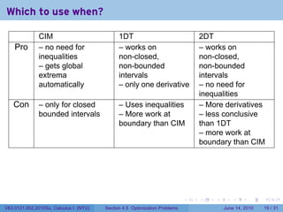
![Recall: The Second Derivative Test
See Section 4.3
Theorem (The Second Derivative Test)
Let f, f′ , and f′′ be continuous on [a, b]. Let c be in (a, b) with f′ (c) = 0.
If f′′ (c) < 0, then f(c) is a local maximum.
If f′′ (c) > 0, then f(c) is a local minimum.
. . . . . .
V63.0121.002.2010Su, Calculus I (NYU) Section 4.5 Optimization Problems June 14, 2010 14 / 31](https://image.slidesharecdn.com/lesson22-optimizationproblemsslides-100615222802-phpapp01-121002230423-phpapp01/85/Lesson22-optimization_problems_slides-32-320.jpg)
![Recall: The Second Derivative Test
See Section 4.3
Theorem (The Second Derivative Test)
Let f, f′ , and f′′ be continuous on [a, b]. Let c be in (a, b) with f′ (c) = 0.
If f′′ (c) < 0, then f(c) is a local maximum.
If f′′ (c) > 0, then f(c) is a local minimum.
Warning
If f′′ (c) = 0, the second derivative test is inconclusive (this does not
mean c is neither; we just don’t know yet).
. . . . . .
V63.0121.002.2010Su, Calculus I (NYU) Section 4.5 Optimization Problems June 14, 2010 14 / 31](https://image.slidesharecdn.com/lesson22-optimizationproblemsslides-100615222802-phpapp01-121002230423-phpapp01/85/Lesson22-optimization_problems_slides-33-320.jpg)
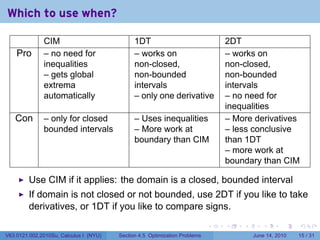
![Recall: The Second Derivative Test
See Section 4.3
Theorem (The Second Derivative Test)
Let f, f′ , and f′′ be continuous on [a, b]. Let c be in (a, b) with f′ (c) = 0.
If f′′ (c) < 0, then f(c) is a local maximum.
If f′′ (c) > 0, then f(c) is a local minimum.
Warning
If f′′ (c) = 0, the second derivative test is inconclusive (this does not
mean c is neither; we just don’t know yet).
Corollary
If f′ (c) = 0 and f′′ (x) > 0 for all x, then c is the global minimum of f
If f′ (c) = 0 and f′′ (x) < 0 for all x, then c is the global maximum of f
. . . . . .
V63.0121.002.2010Su, Calculus I (NYU) Section 4.5 Optimization Problems June 14, 2010 14 / 31](https://image.slidesharecdn.com/lesson22-optimizationproblemsslides-100615222802-phpapp01-121002230423-phpapp01/85/Lesson22-optimization_problems_slides-34-320.jpg)


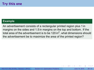
![Solution
1. Everybody understand?
2. Draw a diagram.
3. Length and width are ℓ and w. Length of wire used is p.
4. Q = area = ℓw.
5. Since p = ℓ + 2w, we have ℓ = p − 2w and so
Q(w) = (p − 2w)(w) = pw − 2w2
The domain of Q is [0, p/2]
. . . . . .
V63.0121.002.2010Su, Calculus I (NYU) Section 4.5 Optimization Problems June 14, 2010 24 / 31](https://image.slidesharecdn.com/lesson22-optimizationproblemsslides-100615222802-phpapp01-121002230423-phpapp01/85/Lesson22-optimization_problems_slides-52-320.jpg)
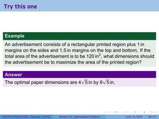
![Solution
1. Everybody understand?
2. Draw a diagram.
3. Length and width are ℓ and w. Length of wire used is p.
4. Q = area = ℓw.
5. Since p = ℓ + 2w, we have ℓ = p − 2w and so
Q(w) = (p − 2w)(w) = pw − 2w2
The domain of Q is [0, p/2]
dQ p
6. = p − 4w, which is zero when w = .
dw 4
. . . . . .
V63.0121.002.2010Su, Calculus I (NYU) Section 4.5 Optimization Problems June 14, 2010 24 / 31](https://image.slidesharecdn.com/lesson22-optimizationproblemsslides-100615222802-phpapp01-121002230423-phpapp01/85/Lesson22-optimization_problems_slides-53-320.jpg)
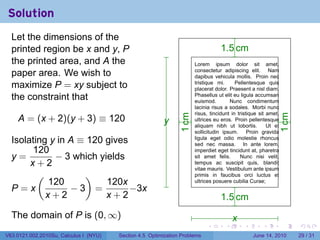
![Solution
1. Everybody understand?
2. Draw a diagram.
3. Length and width are ℓ and w. Length of wire used is p.
4. Q = area = ℓw.
5. Since p = ℓ + 2w, we have ℓ = p − 2w and so
Q(w) = (p − 2w)(w) = pw − 2w2
The domain of Q is [0, p/2]
dQ p
6. = p − 4w, which is zero when w = .
dw 4
. . . . . .
V63.0121.002.2010Su, Calculus I (NYU) Section 4.5 Optimization Problems June 14, 2010 24 / 31](https://image.slidesharecdn.com/lesson22-optimizationproblemsslides-100615222802-phpapp01-121002230423-phpapp01/85/Lesson22-optimization_problems_slides-54-320.jpg)
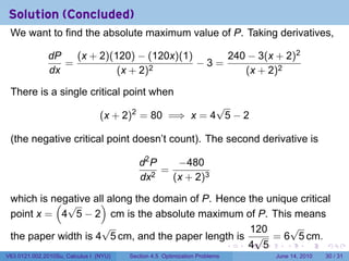
![Solution
1. Everybody understand?
2. Draw a diagram.
3. Length and width are ℓ and w. Length of wire used is p.
4. Q = area = ℓw.
5. Since p = ℓ + 2w, we have ℓ = p − 2w and so
Q(w) = (p − 2w)(w) = pw − 2w2
The domain of Q is [0, p/2]
dQ p
6. = p − 4w, which is zero when w = . Q(0) = Q(p/2) = 0, but
dw 4
(p) p p2 p2
Q =p· −2· = = 80, 000m2
4 4 16 8
so the critical point is the absolute maximum.
. . . . . .
V63.0121.002.2010Su, Calculus I (NYU) Section 4.5 Optimization Problems June 14, 2010 24 / 31](https://image.slidesharecdn.com/lesson22-optimizationproblemsslides-100615222802-phpapp01-121002230423-phpapp01/85/Lesson22-optimization_problems_slides-55-320.jpg)

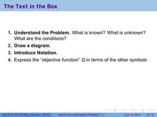
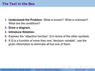
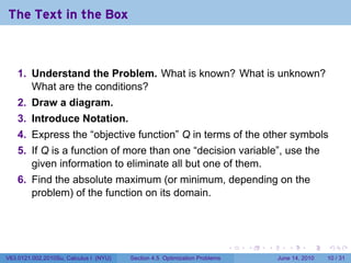
The document summarizes the steps to solve optimization problems using calculus. It begins with an example of finding the rectangle with maximum area given a fixed perimeter. It works through the solution, identifying the objective function, variables, constraints, and using calculus techniques like taking the derivative to find critical points. The document then outlines Polya's 4-step method for problem solving and provides guidance on setting up optimization problems by understanding the problem, introducing notation, drawing diagrams, and eliminating variables using given constraints. It emphasizes using the Closed Interval Method, evaluating the function at endpoints and critical points to determine maximums and minimums.