Downloaded 65 times

![©2007 Pearson Education Asia
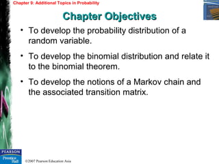
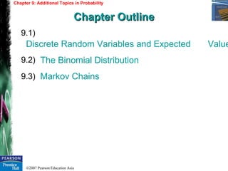
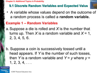
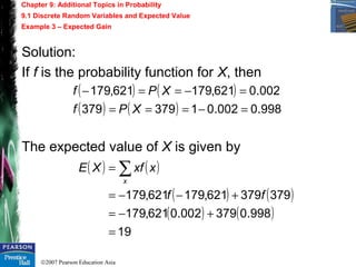
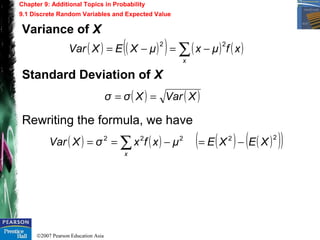
Chapter 9: Additional Topics in Probability
9.1 Discrete Random Variables and Expected Value
Example 1 – Random Variables
c. A student is taking an exam with a one-hour limit.
If X is the number of minutes it takes to complete
the exam, then X is a random variable.
Values that X may assume = (0,60] or 0 < X ≤ 60.
• If X is a discrete random variable with distribution f,
then the mean of X is given by
( ) ( ) ( )∑===
x
xxfXEXμμ](https://image.slidesharecdn.com/introductory-20maths-20analysis-20-20chapter-2009-official-131011125123-phpapp01/85/Introductory-maths-analysis-chapter-09-official-7-320.jpg)

![©2007 Pearson Education Asia
Chapter 9: Additional Topics in Probability
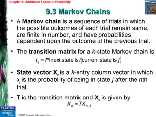
9.3 Markov Chains
Steady-State Vectors
• When T is the k × k transition matrix, the steady-
state vector
is the solution to the matrix equations
=
kq
q
Q
1
[ ]
( ) OQIT
Q
k =−
= 111 ](https://image.slidesharecdn.com/introductory-20maths-20analysis-20-20chapter-2009-official-131011125123-phpapp01/85/Introductory-maths-analysis-chapter-09-official-18-320.jpg)

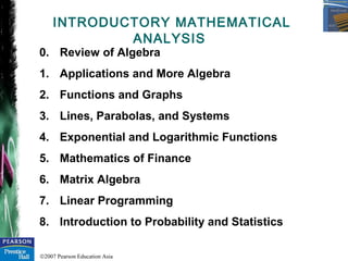
This document summarizes Chapter 9 from a textbook on introductory mathematical analysis. Section 9.1 discusses discrete random variables and expected value. Section 9.2 covers the binomial distribution and how it relates to the binomial theorem. Section 9.3 introduces Markov chains and their associated transition matrices. Examples are provided for each topic to illustrate key concepts like calculating expected values, applying the binomial distribution formula, and determining probabilities using Markov chains.