Downloaded 143 times


![The definite integral as a limit
Definition
If f is a function defined on [a, b], the definite integral of f from a to b
is the number ∫ b ∑n
f(x) dx = lim f(ci ) ∆x
a ∆x→0
i=1
. . . . . .
V63.0121.006/016, Calculus I (NYU) Section 5.4 The Fundamental Theorem April 22, 2010 6 / 34](https://image.slidesharecdn.com/lesson25-thefundamentaltheoremofcalculusslides-100422151022-phpapp01/75/Lesson-25-The-Fundamental-Theorem-of-Calculus-7-2048.jpg)
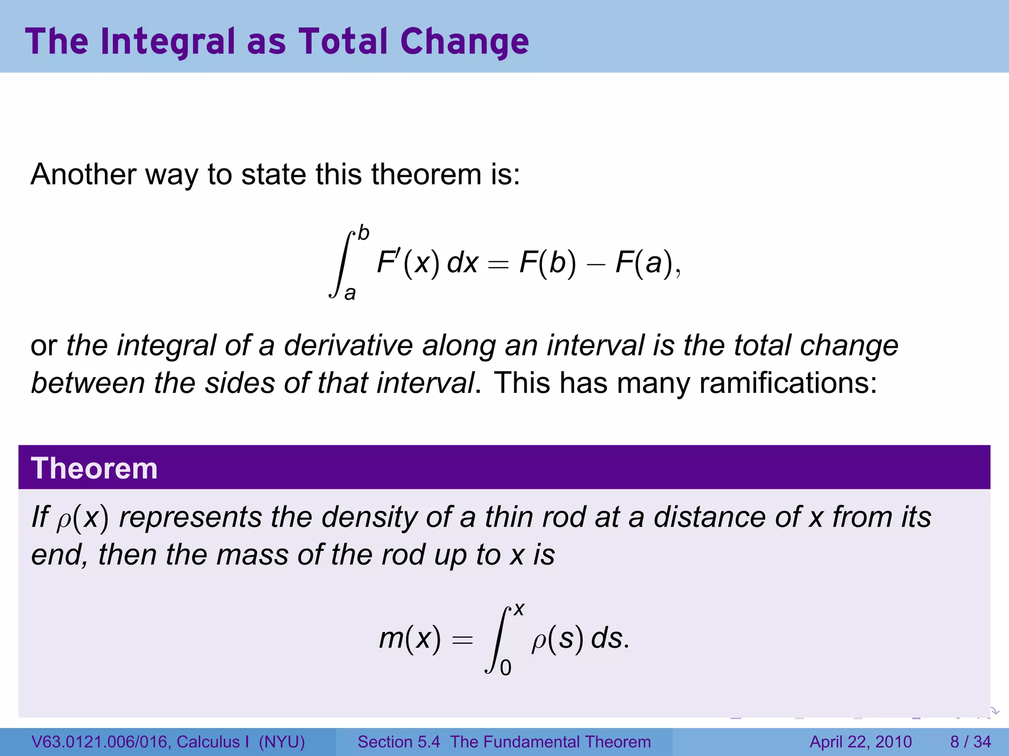
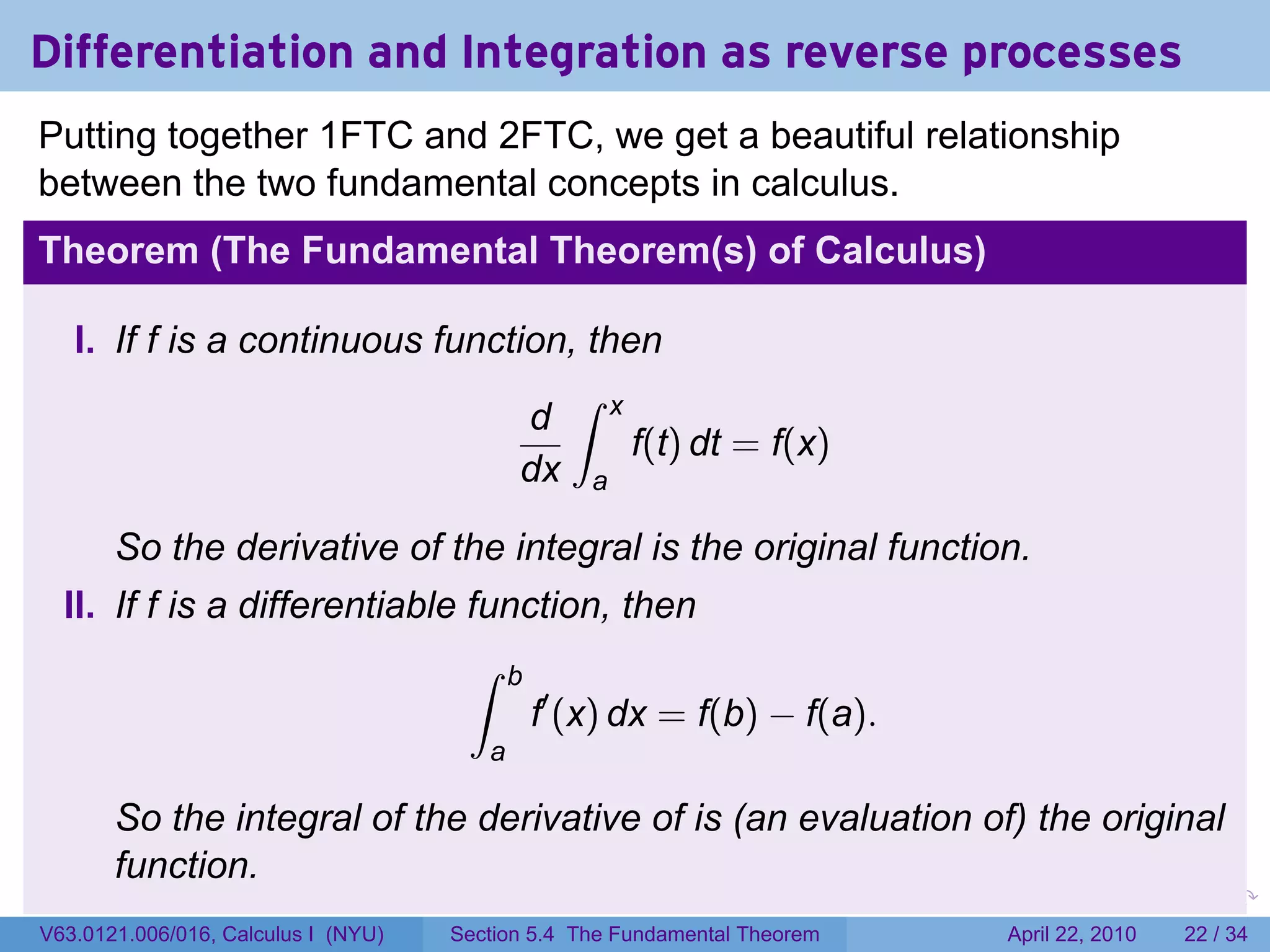
![Theorem (The Second Fundamental Theorem of Calculus)
Suppose f is integrable on [a, b] and f = F′ for another function F, then
∫ b
f(x) dx = F(b) − F(a).
a
. . . . . .
V63.0121.006/016, Calculus I (NYU) Section 5.4 The Fundamental Theorem April 22, 2010 7 / 34](https://image.slidesharecdn.com/lesson25-thefundamentaltheoremofcalculusslides-100422151022-phpapp01/75/Lesson-25-The-Fundamental-Theorem-of-Calculus-8-2048.jpg)
![My first table of integrals
.
∫ ∫ ∫
[f(x) + g(x)] dx = f(x) dx + g(x) dx
∫ ∫ ∫
xn+1
xn dx = + C (n ̸= −1) cf(x) dx = c f(x) dx
n+1 ∫
∫
1
ex dx = ex + C dx = ln |x| + C
x
∫ ∫
ax
sin x dx = − cos x + C ax dx = +C
ln a
∫ ∫
cos x dx = sin x + C csc2 x dx = − cot x + C
∫ ∫
2
sec x dx = tan x + C csc x cot x dx = − csc x + C
∫ ∫
1
sec x tan x dx = sec x + C √ dx = arcsin x + C
∫ 1 − x2
1
dx = arctan x + C
1 + x2
. . . . . . .
V63.0121.006/016, Calculus I (NYU) Section 5.4 The Fundamental Theorem April 22, 2010 9 / 34](https://image.slidesharecdn.com/lesson25-thefundamentaltheoremofcalculusslides-100422151022-phpapp01/75/Lesson-25-The-Fundamental-Theorem-of-Calculus-13-2048.jpg)
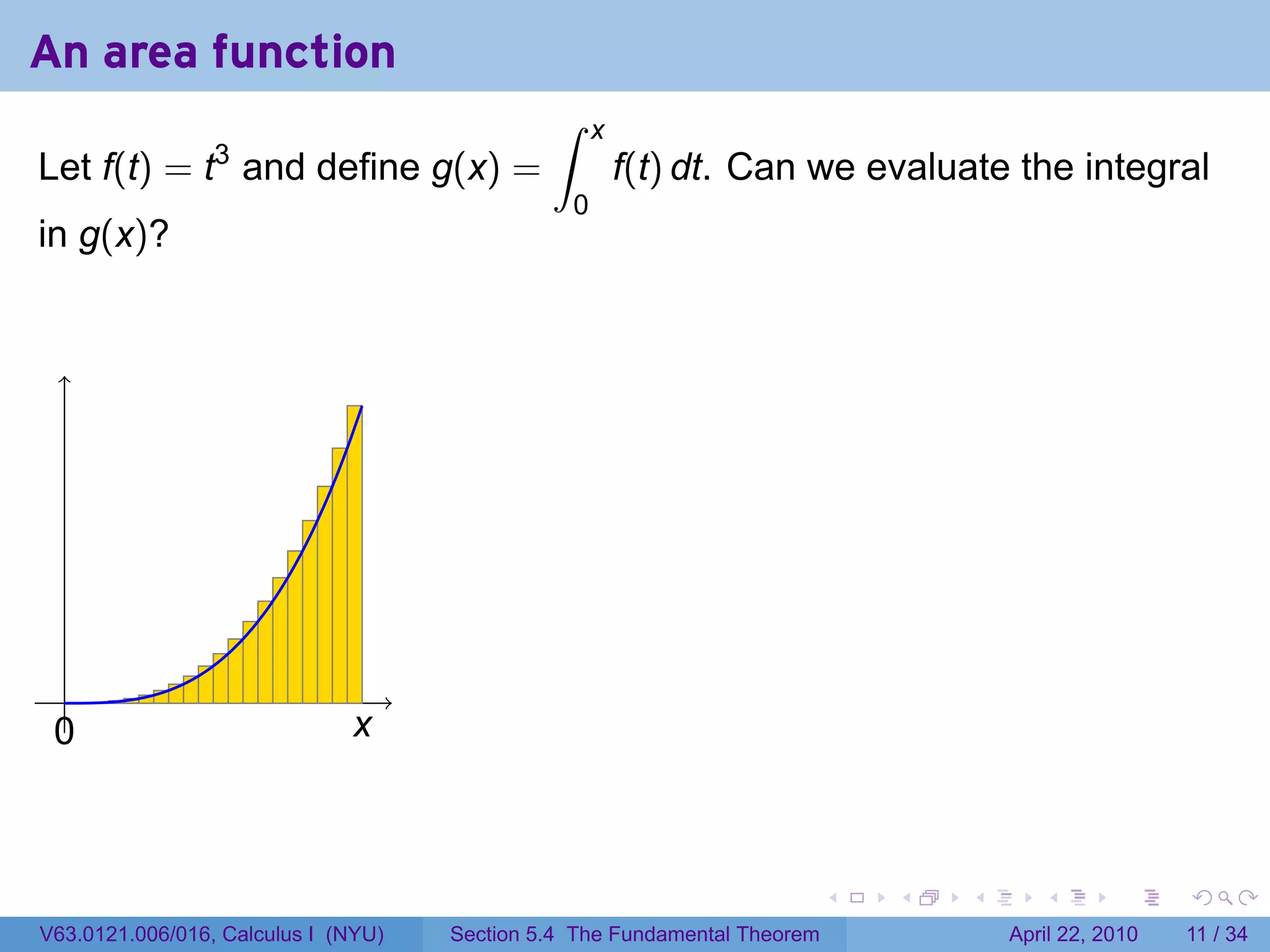
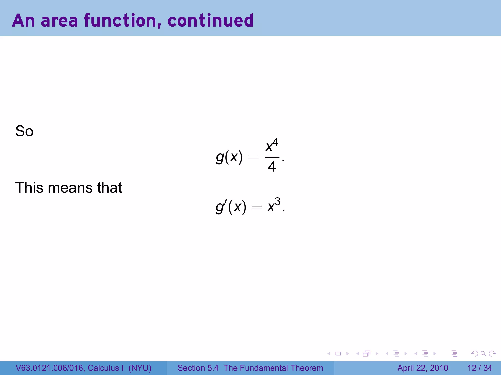
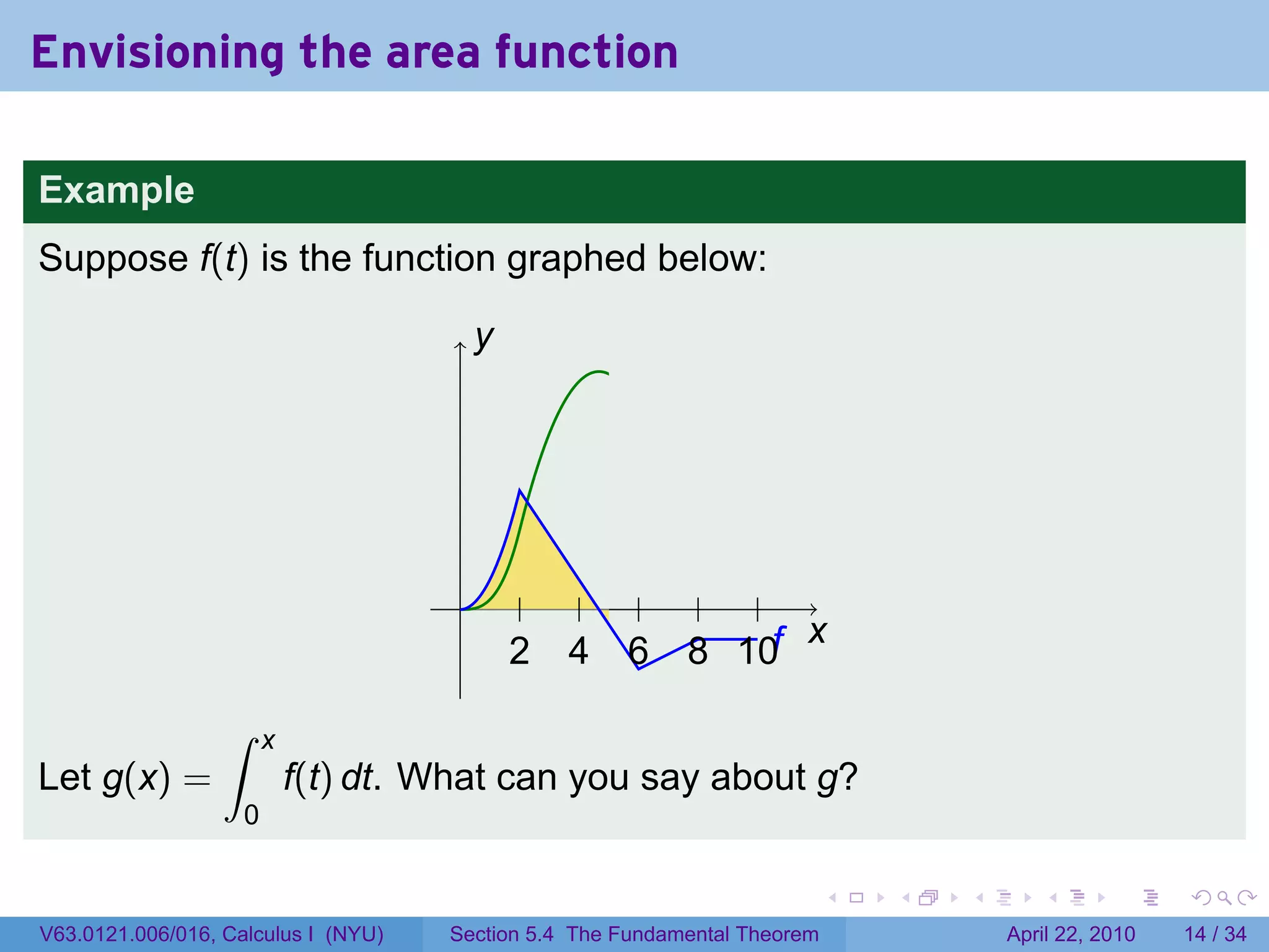
![An area function
∫ x
Let f(t) = t3 and define g(x) = f(t) dt. Can we evaluate the integral
0
in g(x)?
Dividing the interval [0, x] into n pieces
x ix
gives ∆t = and ti = 0 + i∆t = . So
n n
x x3 x (2x)3 x (nx)3
Rn = · 3+ · + ··· + ·
n n n n3 n n3
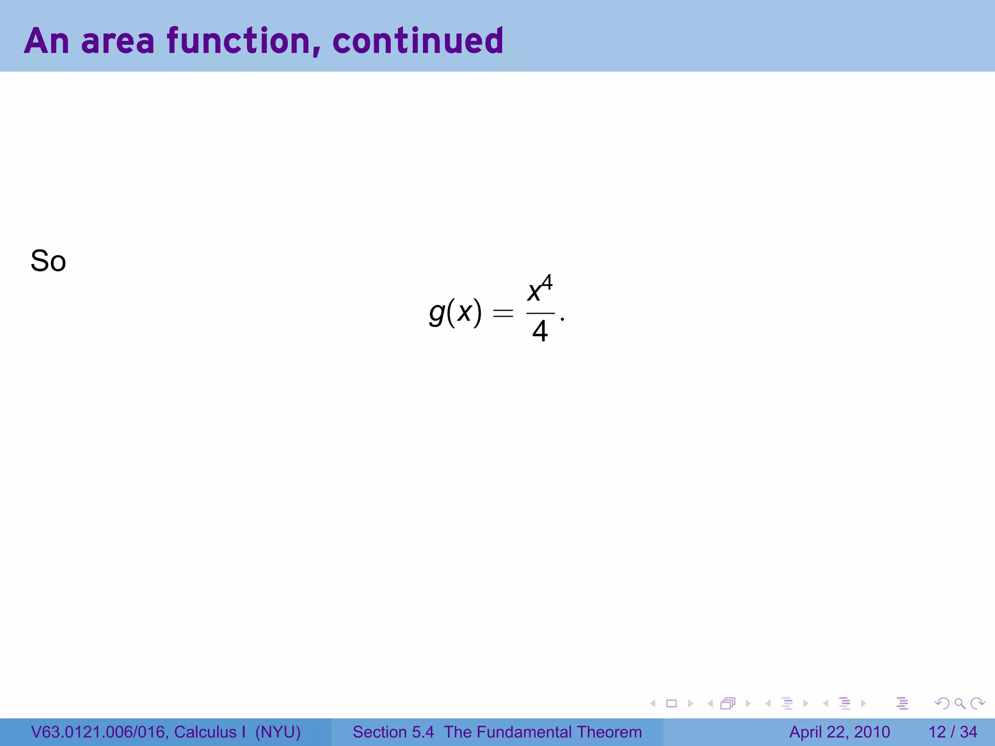
x4 ( )
= 4 13 + 23 + 33 + · · · + n3
n
x4 [ ]2
= 4 1 n(n + 1)
. n 2
0
. x
.
x4 n2 (n + 1)2 x4
= →
4n4 4
as n → ∞.
. . . . . .
V63.0121.006/016, Calculus I (NYU) Section 5.4 The Fundamental Theorem April 22, 2010 11 / 34](https://image.slidesharecdn.com/lesson25-thefundamentaltheoremofcalculusslides-100422151022-phpapp01/75/Lesson-25-The-Fundamental-Theorem-of-Calculus-16-2048.jpg)
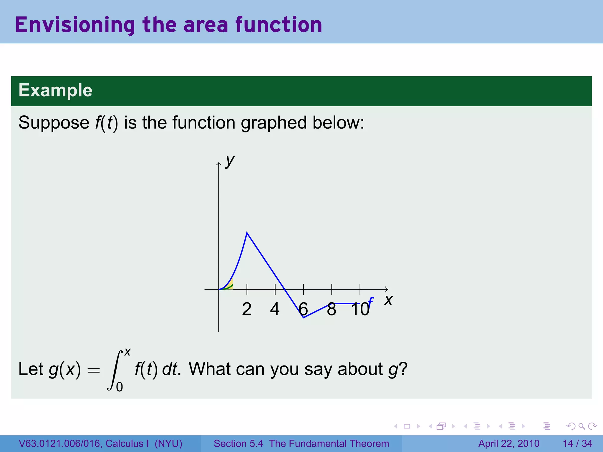
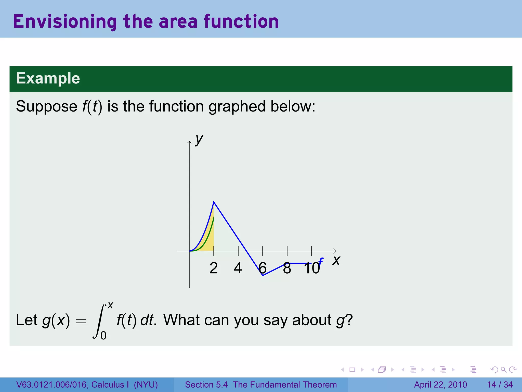
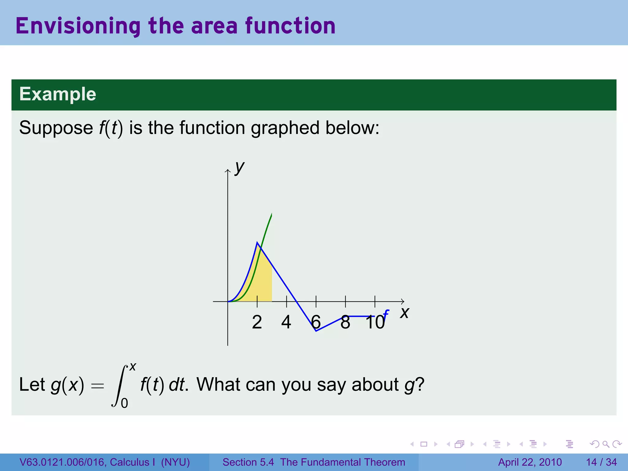
![The area function
Let f be a function which is integrable (i.e., continuous or with finitely
many jump discontinuities) on [a, b]. Define
∫ x
g(x) = f(t) dt.
a
The variable is x; t is a “dummy” variable that’s integrated over.
Picture changing x and taking more of less of the region under the
curve.
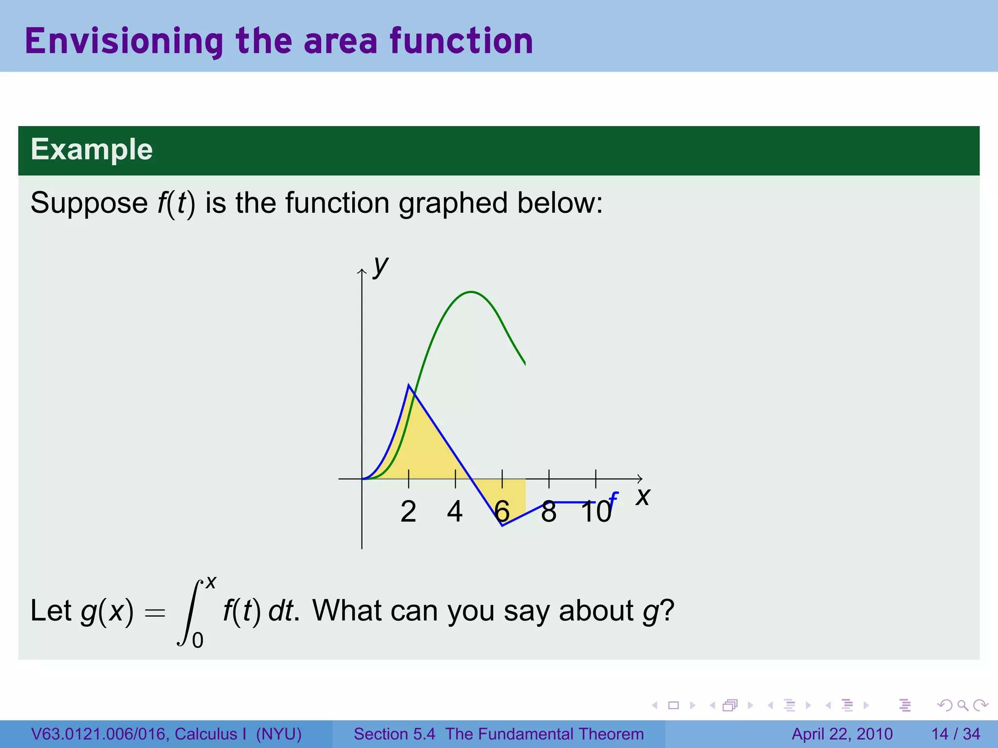
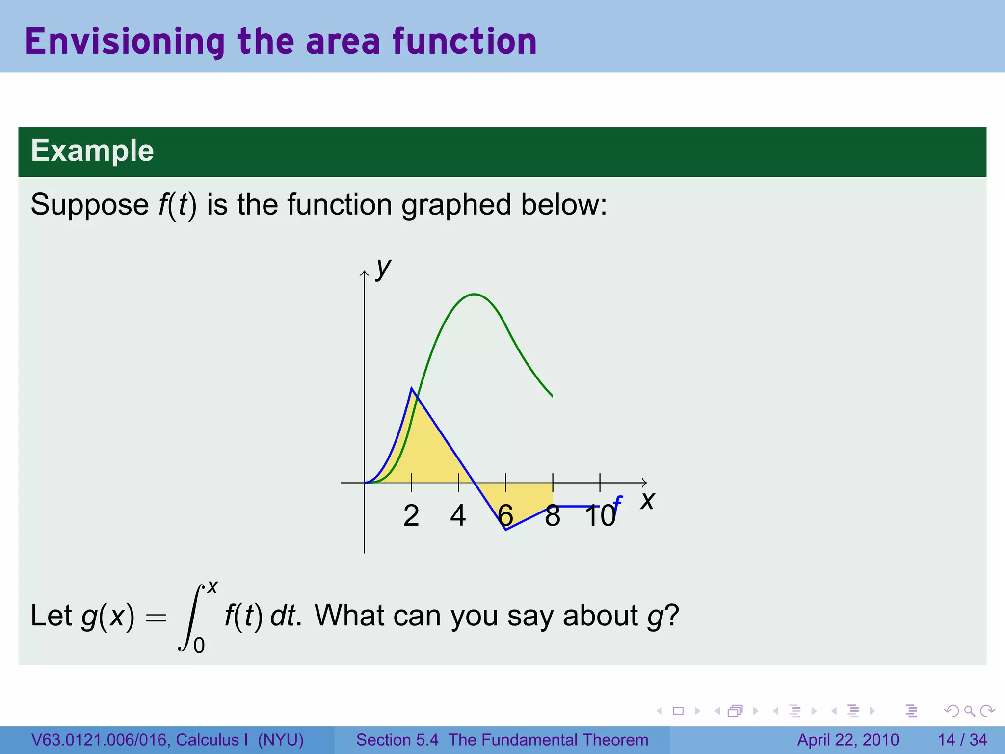
Question: What does f tell you about g?
. . . . . .
V63.0121.006/016, Calculus I (NYU) Section 5.4 The Fundamental Theorem April 22, 2010 13 / 34](https://image.slidesharecdn.com/lesson25-thefundamentaltheoremofcalculusslides-100422151022-phpapp01/75/Lesson-25-The-Fundamental-Theorem-of-Calculus-19-2048.jpg)


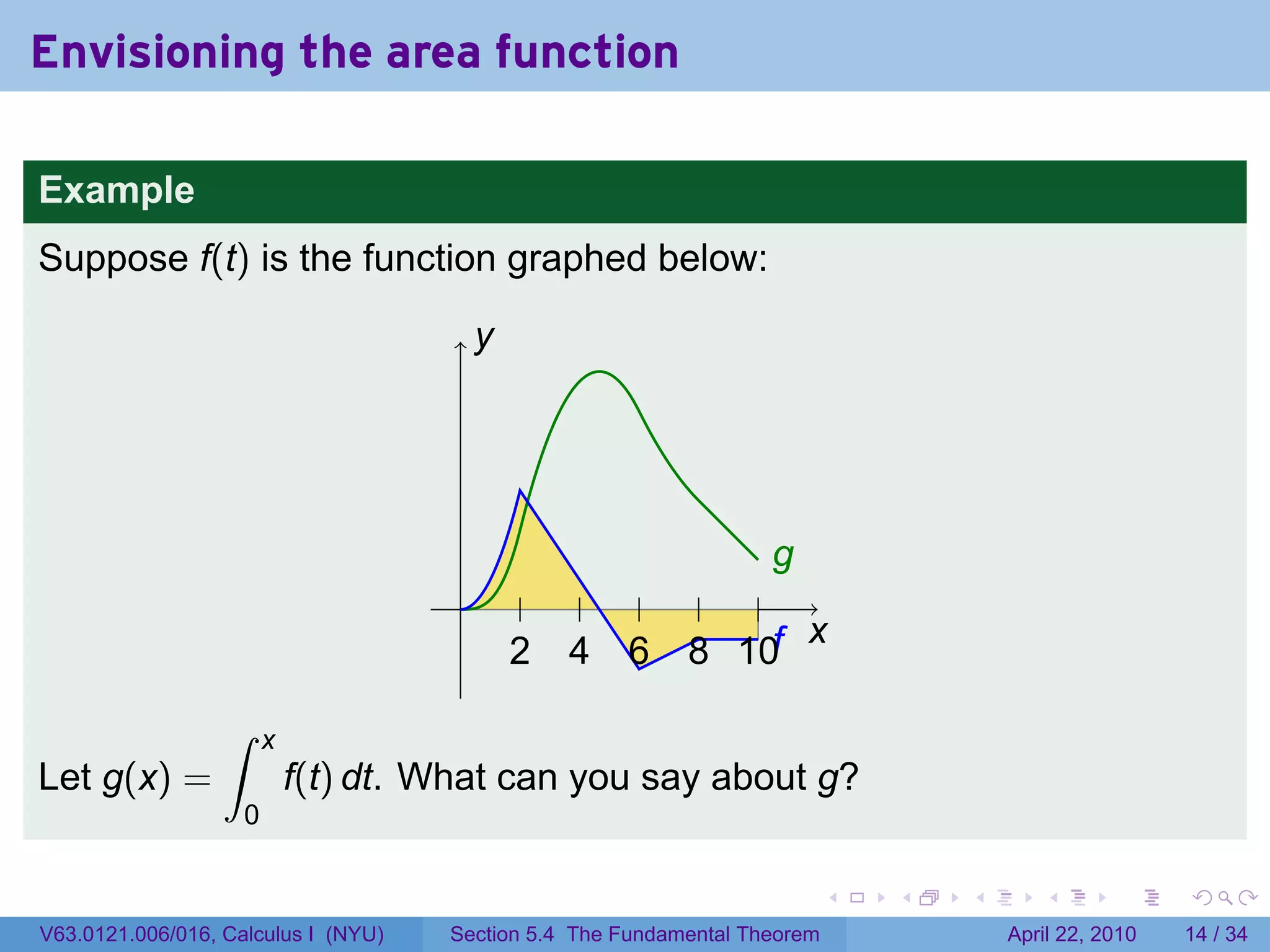
![features of g from f
..
y
Interval sign monotonicity monotonicity concavity
. of f of g of f of g
g
.
. . . . . . . [0, 2] + ↗ ↗ ⌣
. ..fx
. . .. . . 0
2 4 6 81 [2, 4.5] + ↗ ↘ ⌢
[4.5, 6] − ↘ ↘ ⌢
[6, 8] − ↘ ↗ ⌣
[8, 10] − ↘ → none
. . . . . .
V63.0121.006/016, Calculus I (NYU) Section 5.4 The Fundamental Theorem April 22, 2010 15 / 34](https://image.slidesharecdn.com/lesson25-thefundamentaltheoremofcalculusslides-100422151022-phpapp01/75/Lesson-25-The-Fundamental-Theorem-of-Calculus-32-2048.jpg)
![features of g from f
..
y
Interval sign monotonicity monotonicity concavity
. of f of g of f of g
g
.
. . . . . . . [0, 2] + ↗ ↗ ⌣
. ..fx
. . .. . . 0
2 4 6 81 [2, 4.5] + ↗ ↘ ⌢
[4.5, 6] − ↘ ↘ ⌢
[6, 8] − ↘ ↗ ⌣
[8, 10] − ↘ → none
We see that g is behaving a lot like an antiderivative of f.
. . . . . .
V63.0121.006/016, Calculus I (NYU) Section 5.4 The Fundamental Theorem April 22, 2010 15 / 34](https://image.slidesharecdn.com/lesson25-thefundamentaltheoremofcalculusslides-100422151022-phpapp01/75/Lesson-25-The-Fundamental-Theorem-of-Calculus-33-2048.jpg)
![Theorem (The First Fundamental Theorem of Calculus)
Let f be an integrable function on [a, b] and define
∫ x
g(x) = f(t) dt.
a
If f is continuous at x in (a, b), then g is differentiable at x and
g′ (x) = f(x).
. . . . . .
V63.0121.006/016, Calculus I (NYU) Section 5.4 The Fundamental Theorem April 22, 2010 16 / 34](https://image.slidesharecdn.com/lesson25-thefundamentaltheoremofcalculusslides-100422151022-phpapp01/75/Lesson-25-The-Fundamental-Theorem-of-Calculus-34-2048.jpg)
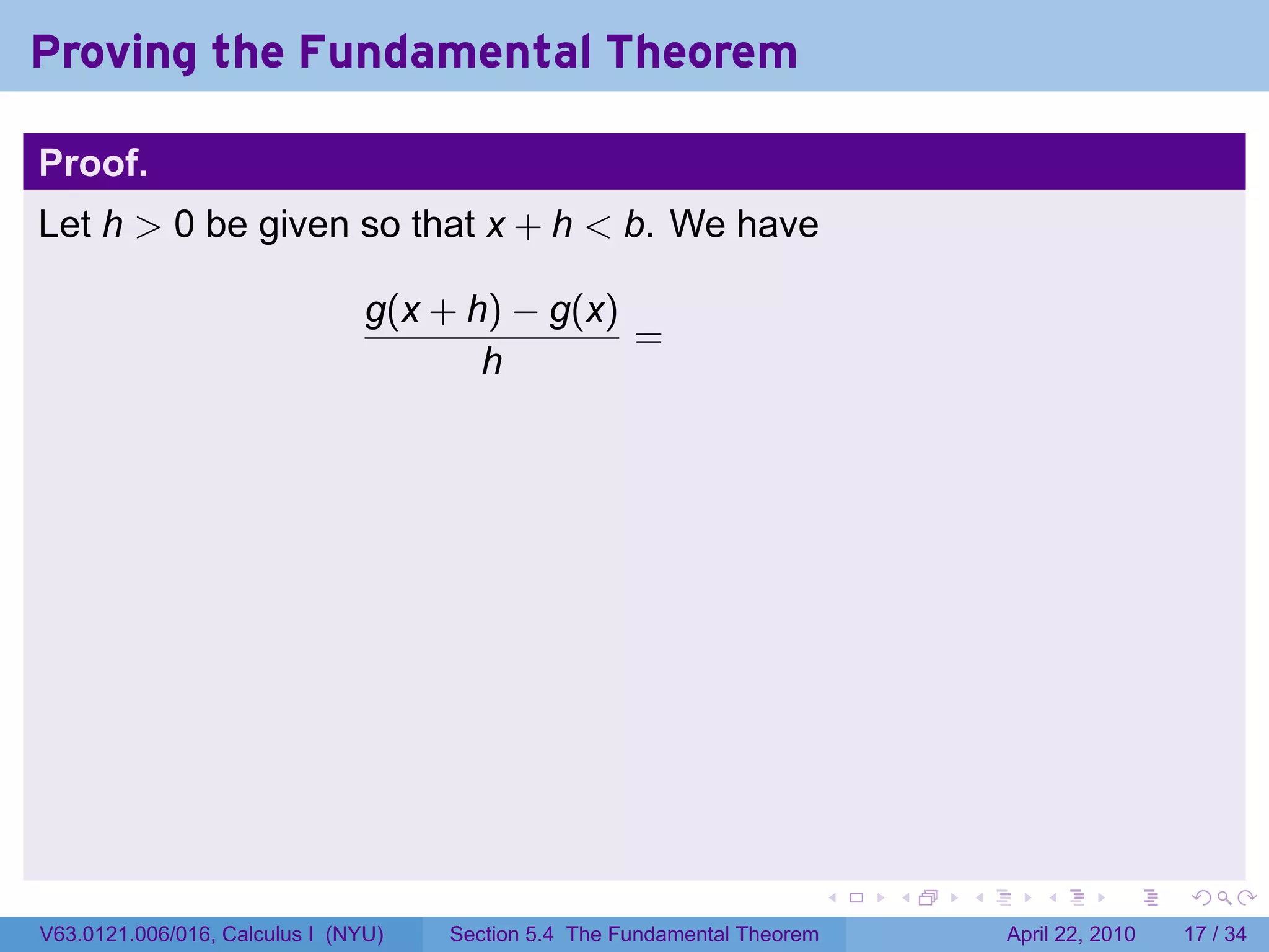
![Proving the Fundamental Theorem
Proof.
Let h > 0 be given so that x + h < b. We have
∫
g(x + h) − g(x) 1 x+h
= f(t) dt.
h h x
Let Mh be the maximum value of f on [x, x + h], and let mh the minimum
value of f on [x, x + h]. From §5.2 we have
∫ x+h
f(t) dt
x
So
g(x + h) − g(x)
mh ≤ ≤ Mh .
h
. . . . . .
V63.0121.006/016, Calculus I (NYU) Section 5.4 The Fundamental Theorem April 22, 2010 17 / 34](https://image.slidesharecdn.com/lesson25-thefundamentaltheoremofcalculusslides-100422151022-phpapp01/75/Lesson-25-The-Fundamental-Theorem-of-Calculus-37-2048.jpg)
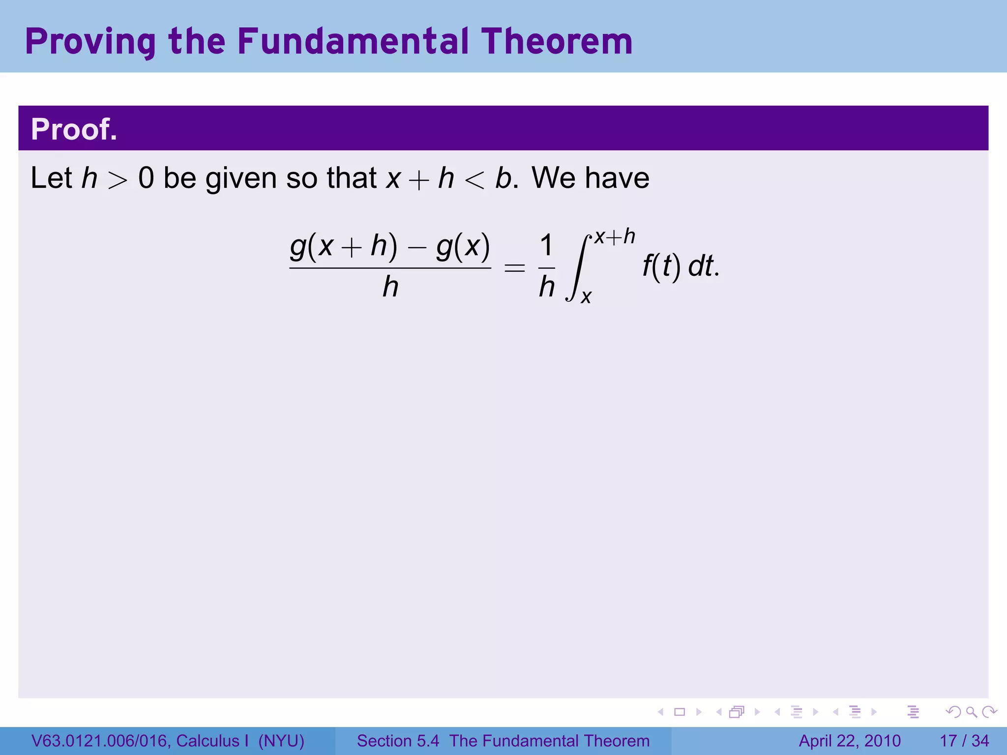
![Proving the Fundamental Theorem
Proof.
Let h > 0 be given so that x + h < b. We have
∫
g(x + h) − g(x) 1 x+h
= f(t) dt.
h h x
Let Mh be the maximum value of f on [x, x + h], and let mh the minimum
value of f on [x, x + h]. From §5.2 we have
∫ x+h
f(t) dt ≤ Mh · h
x
So
g(x + h) − g(x)
mh ≤ ≤ Mh .
h
As h → 0, both mh and Mh tend to f(x).
. . . . . .
V63.0121.006/016, Calculus I (NYU) Section 5.4 The Fundamental Theorem April 22, 2010 17 / 34](https://image.slidesharecdn.com/lesson25-thefundamentaltheoremofcalculusslides-100422151022-phpapp01/75/Lesson-25-The-Fundamental-Theorem-of-Calculus-38-2048.jpg)
![Proving the Fundamental Theorem
Proof.
Let h > 0 be given so that x + h < b. We have
∫
g(x + h) − g(x) 1 x+h
= f(t) dt.
h h x
Let Mh be the maximum value of f on [x, x + h], and let mh the minimum
value of f on [x, x + h]. From §5.2 we have
∫ x+h
mh · h ≤ f(t) dt ≤ Mh · h
x
So
g(x + h) − g(x)
mh ≤ ≤ Mh .
h
As h → 0, both mh and Mh tend to f(x).
. . . . . .
V63.0121.006/016, Calculus I (NYU) Section 5.4 The Fundamental Theorem April 22, 2010 17 / 34](https://image.slidesharecdn.com/lesson25-thefundamentaltheoremofcalculusslides-100422151022-phpapp01/75/Lesson-25-The-Fundamental-Theorem-of-Calculus-39-2048.jpg)


The document is a lecture note on the fundamental theorem of calculus from a Calculus I class at New York University. It provides announcements about upcoming exams and assignments. It then outlines the key topics to be covered, including the first fundamental theorem of calculus and how to differentiate functions defined by integrals. Examples are provided to illustrate using integrals to find the area under a curve and how this relates to the derivative of the area function.