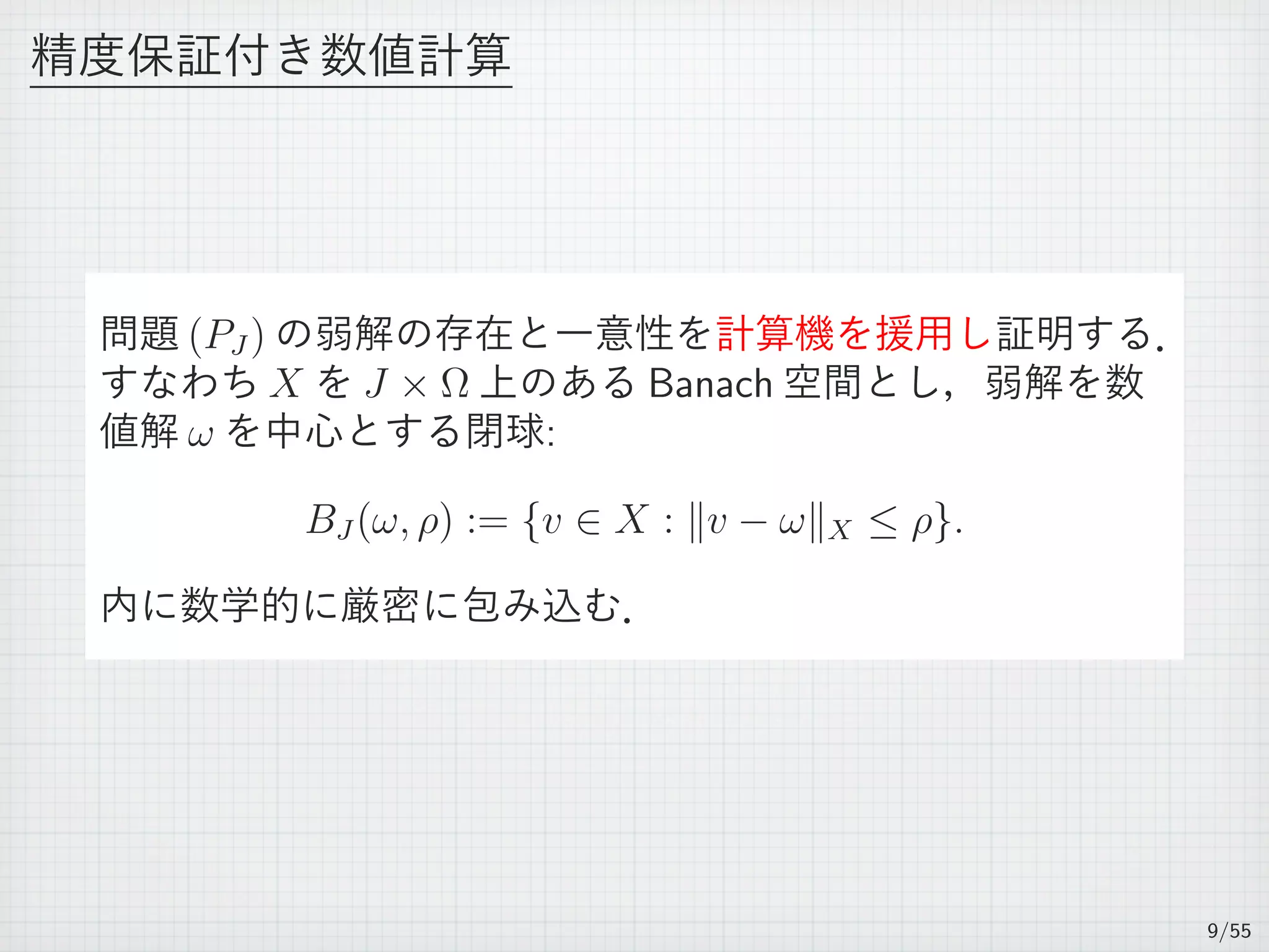
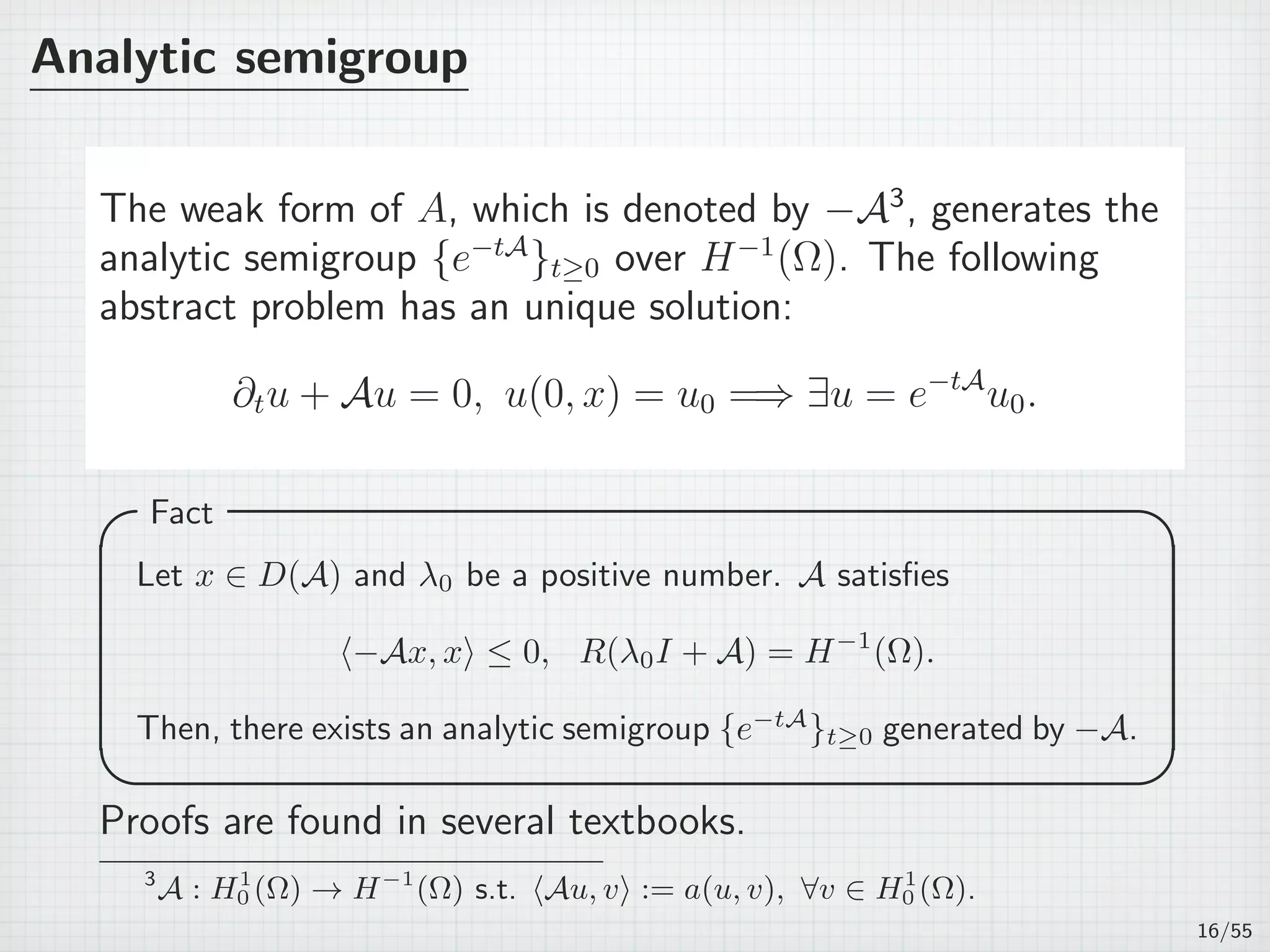
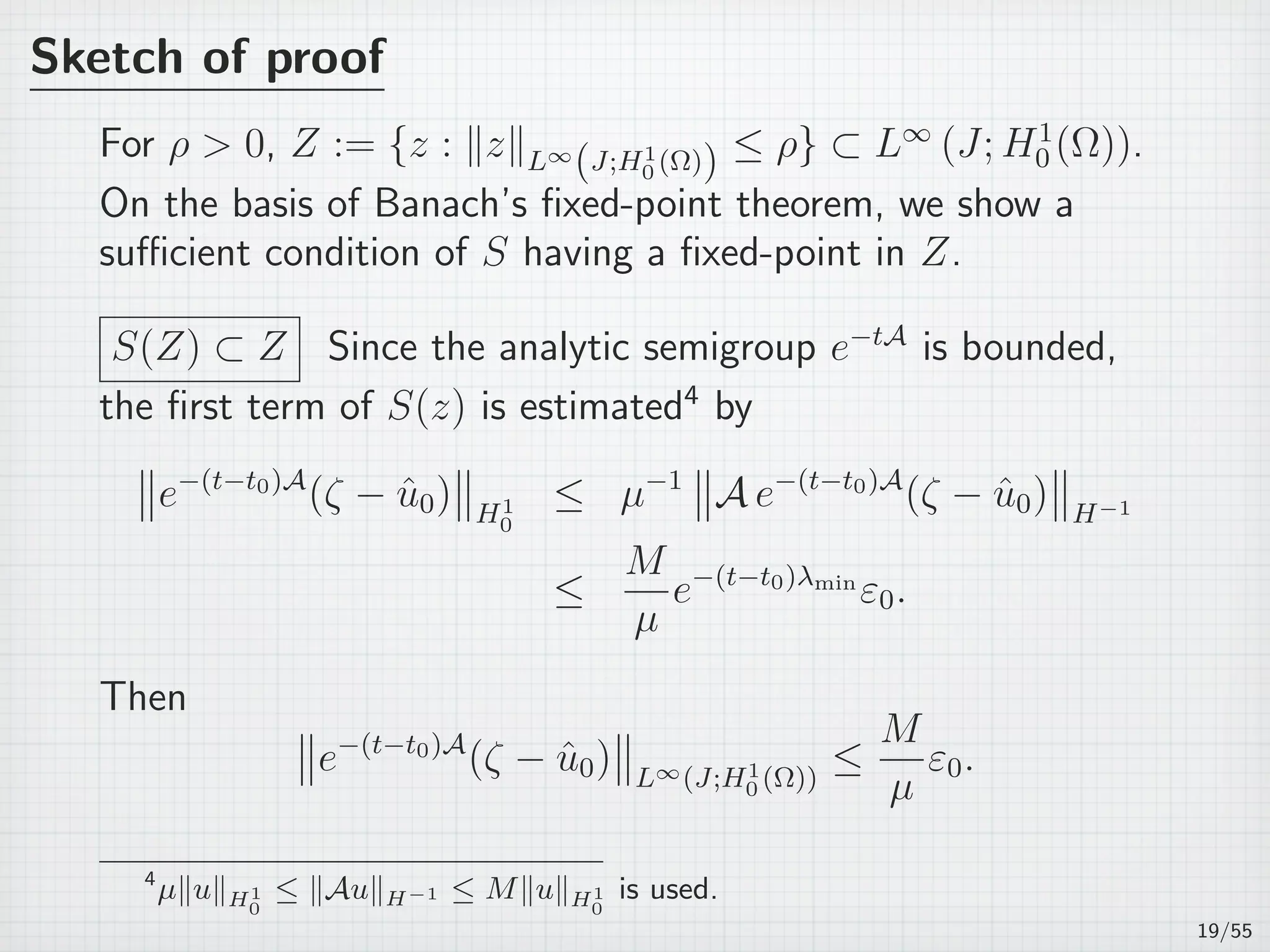
This document summarizes a presentation on rigorously verifying the accuracy of numerical solutions to semi-linear parabolic partial differential equations using analytic semigroups. It introduces the considered problem of finding the solution to a semi-linear parabolic PDE. It then discusses using a piecewise linear finite element discretization in space and time to obtain an initial numerical solution. The goal is to rigorously enclose the true solution within a radius ρ of this numerical solution in the function space L∞(J;H10(Ω)). Key steps involve using properties of the analytic semigroup generated by the operator A and estimating discretization errors to compute the enclosure radius ρ.

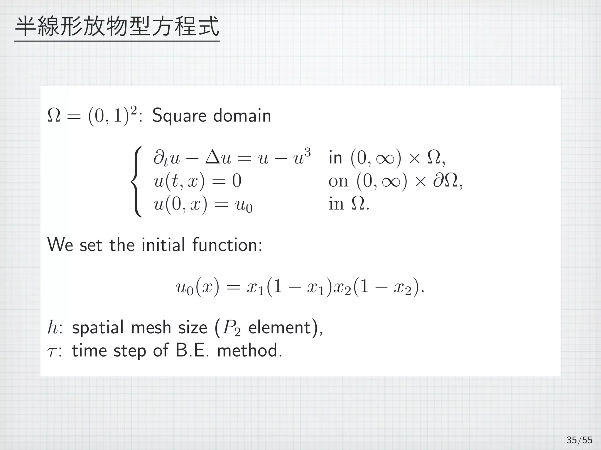
![半線形放物型方程式
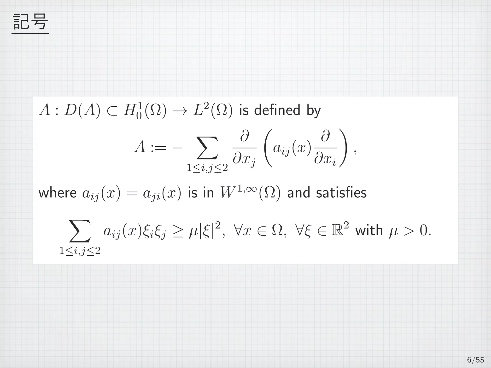
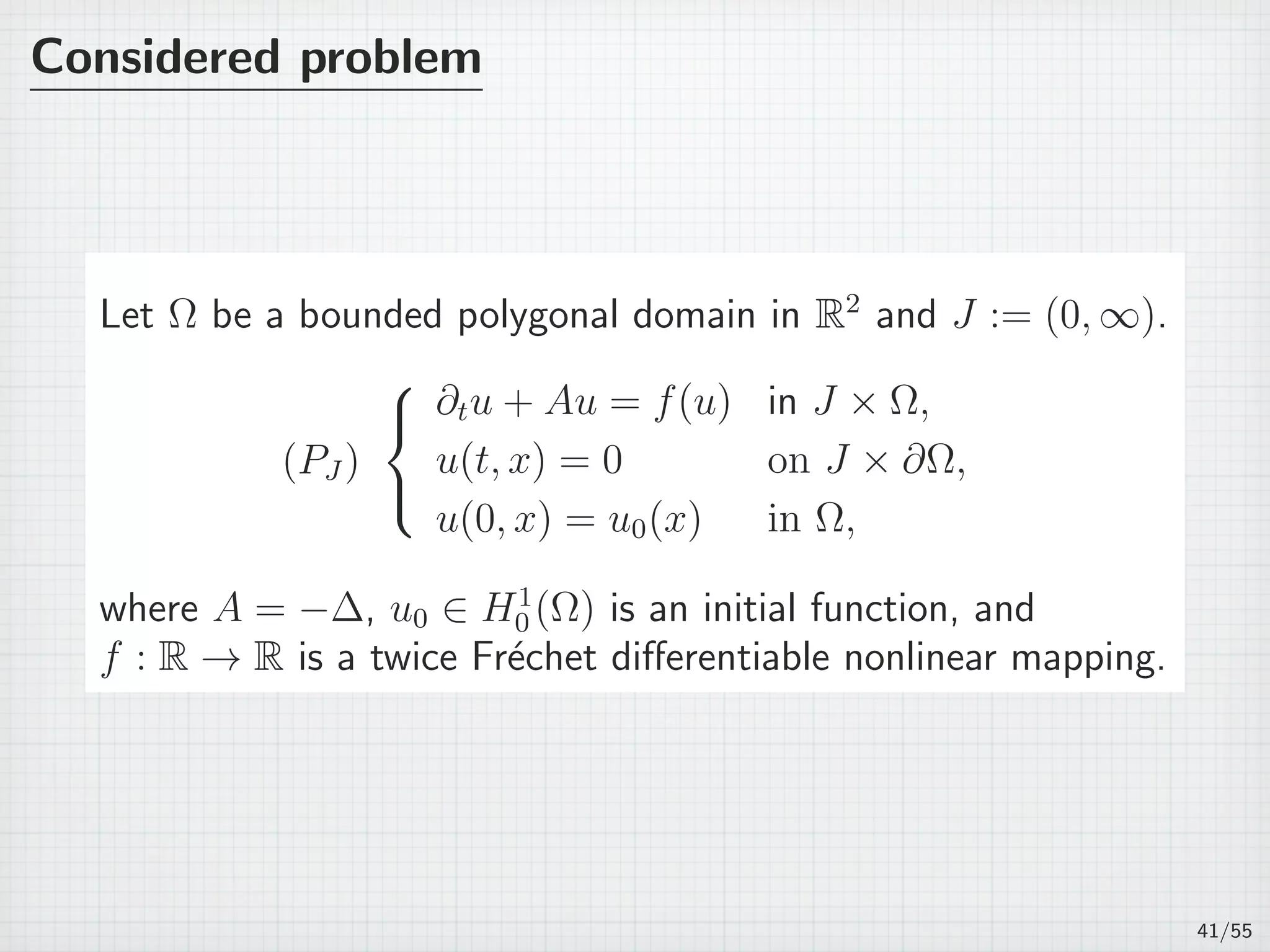
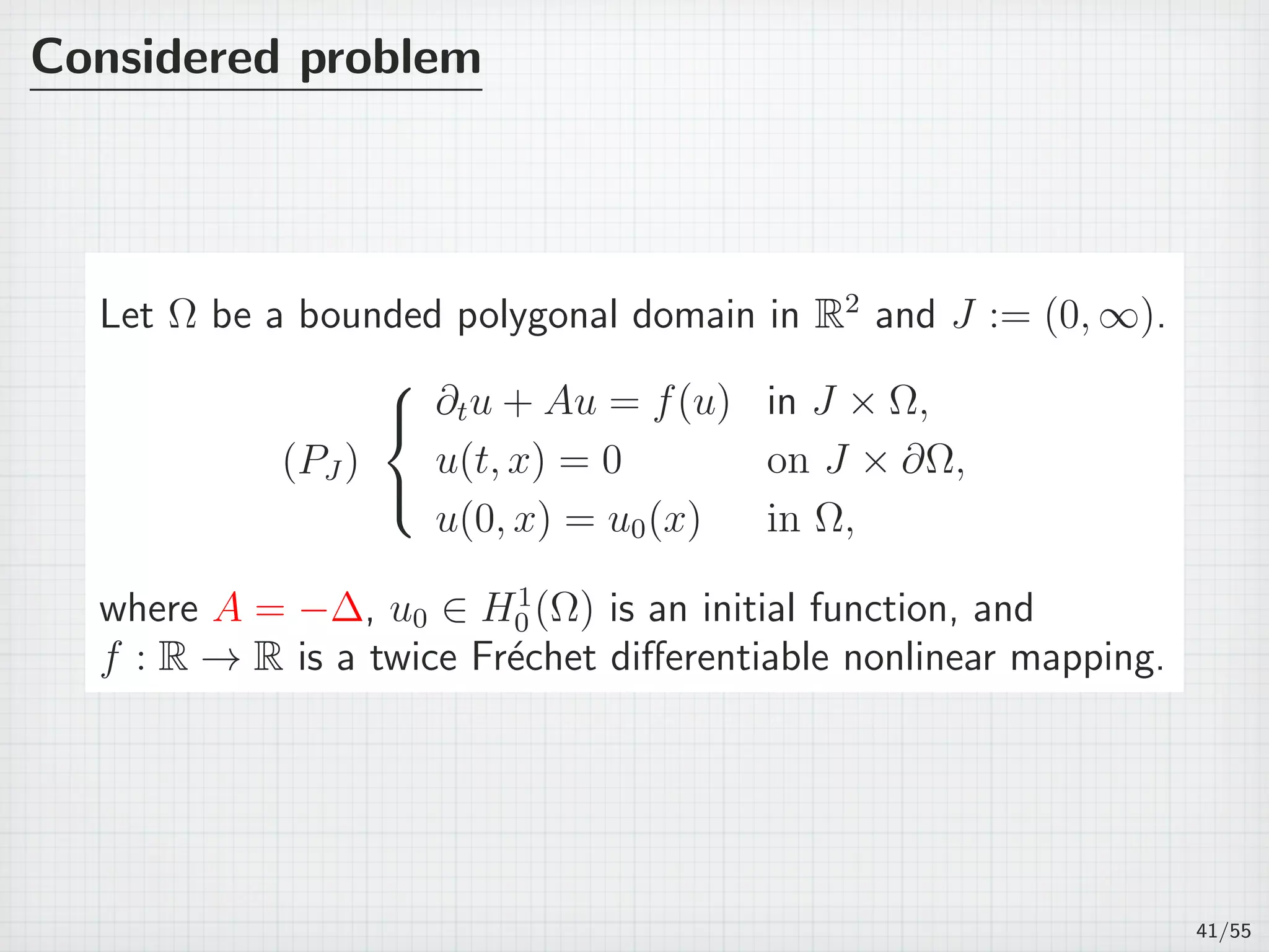
Let Ω be a bounded polygonal domain in R2
.
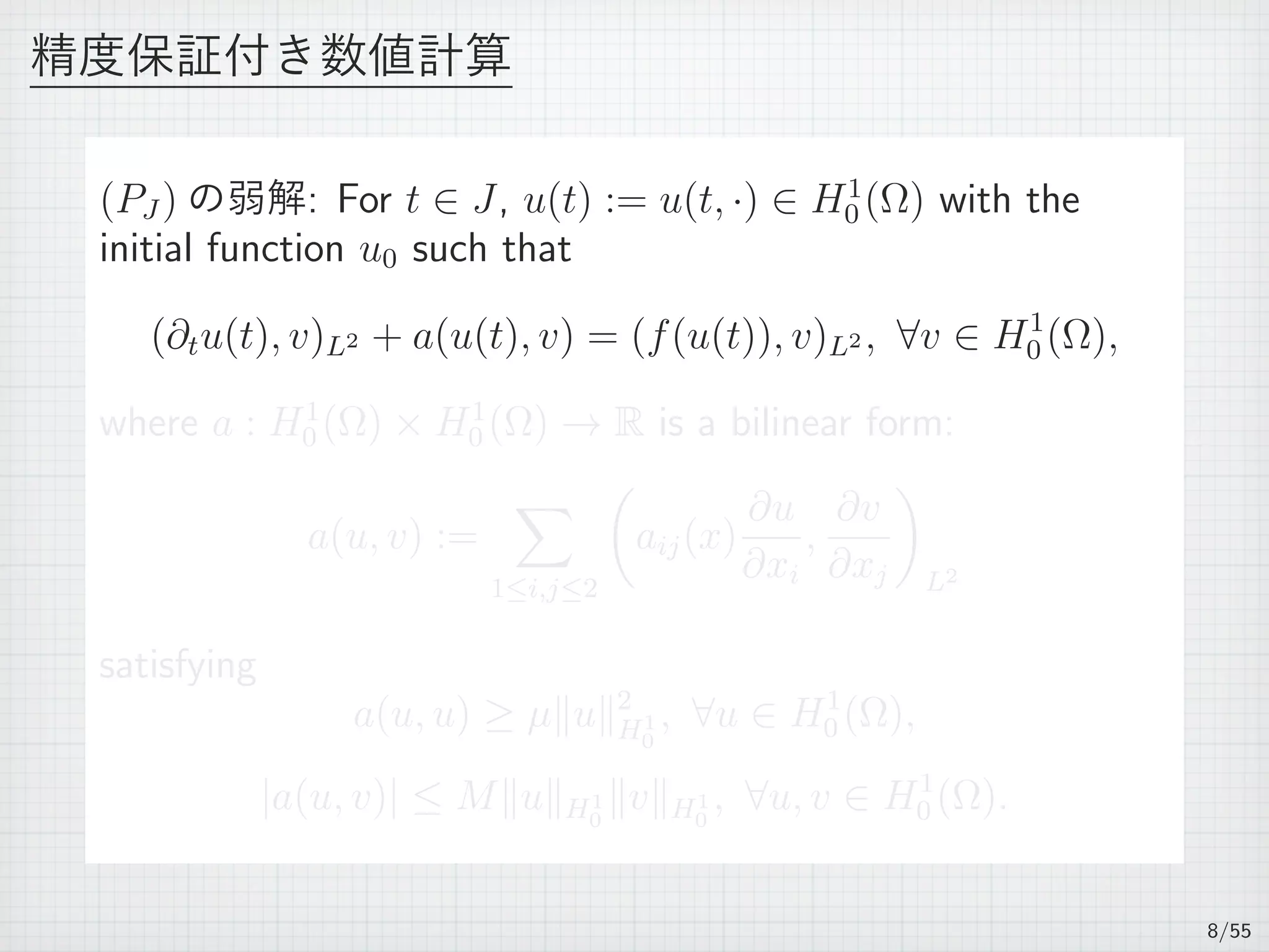
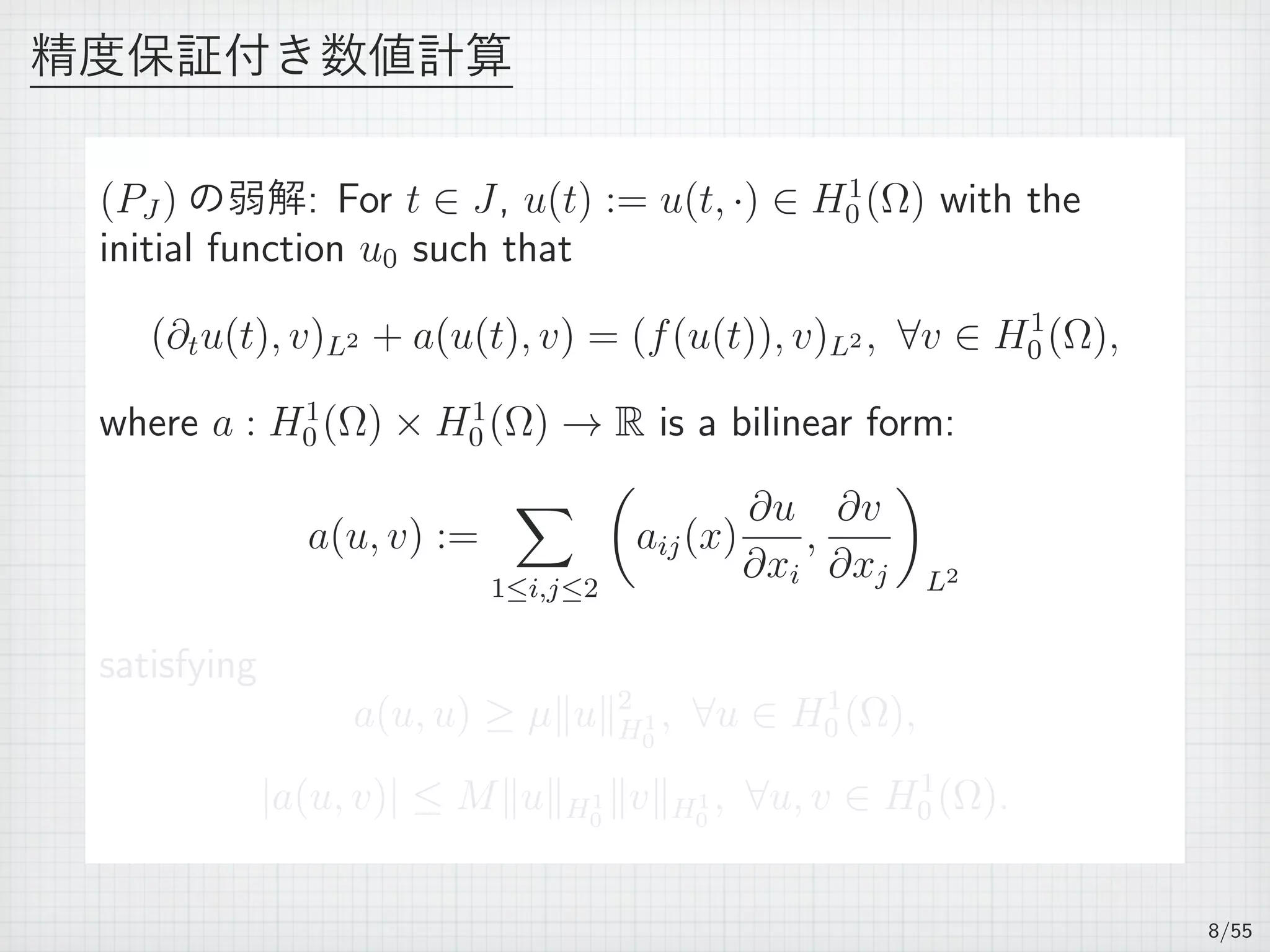
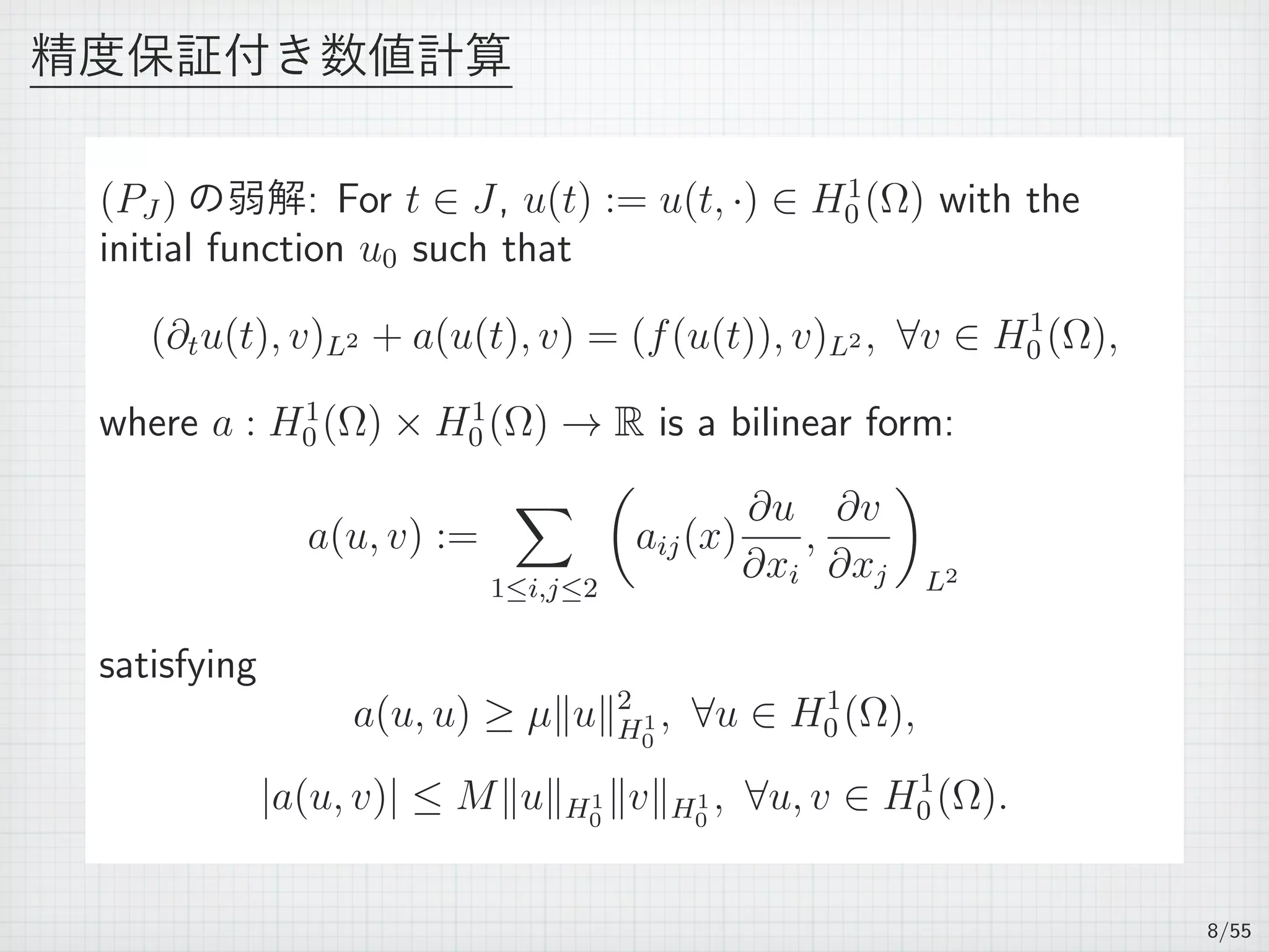
(PJ )
∂tu + Au = f(u) in J × Ω,
u(t, x) = 0 on J × ∂Ω,
u(t0, x) = u0(x) in Ω,
▶ J := (t0, t1], 0 ≤ t0 < t1 < ∞ or J := (0, ∞),
▶ f : twice differentiable nonlinear mapping,
▶ u = 0 on ∂Ω is the trace sense,
▶ u0 ∈ H1
0 (Ω).
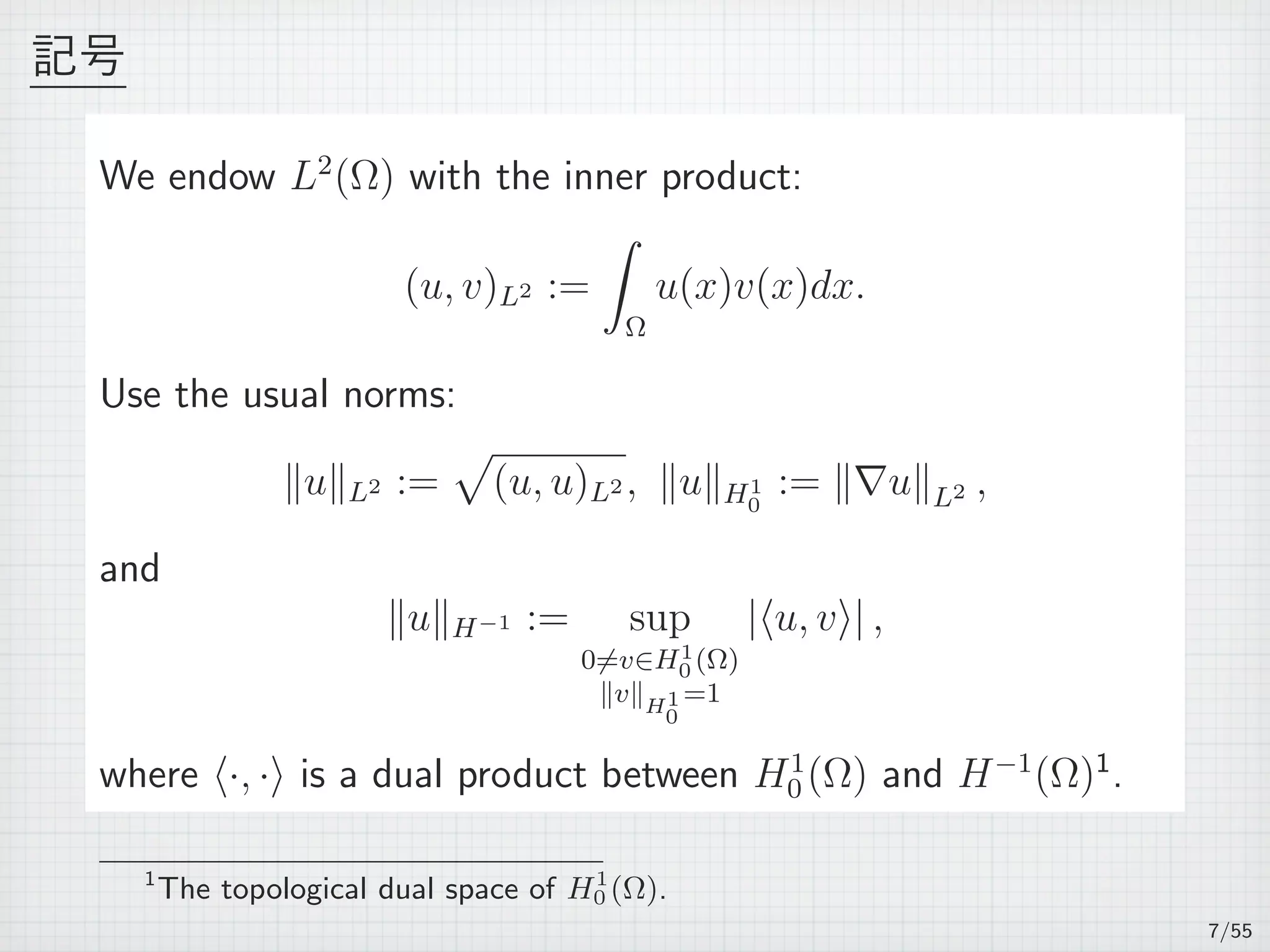
Lp
(Ω): the set of Lp
-functions,
H1
(Ω): the first order Sobolev space of L2
(Ω),
H1
0 (Ω) := {v ∈ H1
(Ω) : v = 0 on ∂Ω}.
5/55](https://image.slidesharecdn.com/akitoshitakayasu-160128011103/75/Akitoshi-Takayasu-5-2048.jpg)

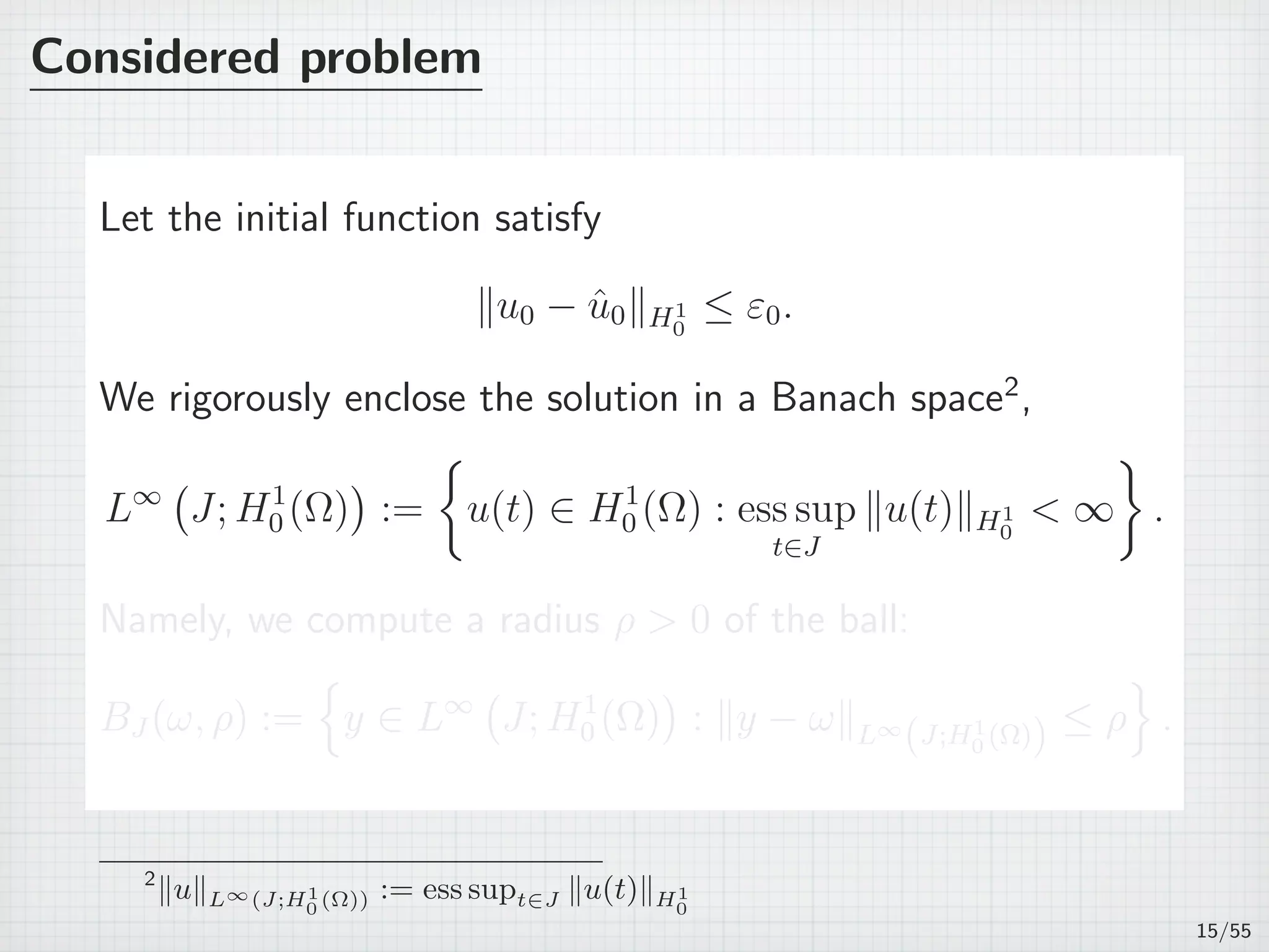
![Considered problem
J := (t0, t1] : arbitrary time interval. τ := t1 − t0.
(PJ )
∂tu + Au = f(u) in J × Ω,
u(t, x) = 0 on J × ∂Ω,
u(t0, x) = u0(x) in Ω,
where u0 is an initial function in H1
0 (Ω).
Vh ⊂ H1
0 (Ω) : a finite dimensional subspace.
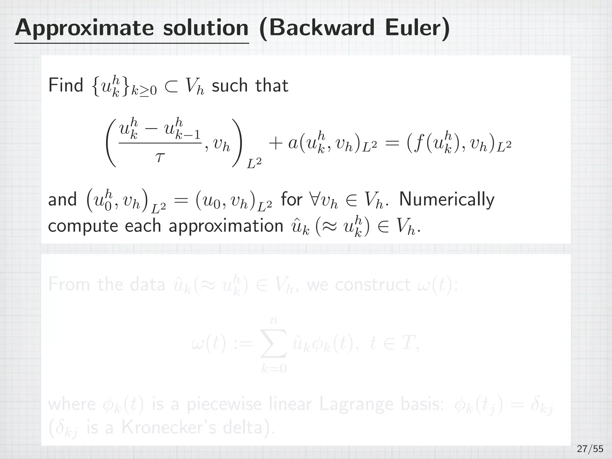
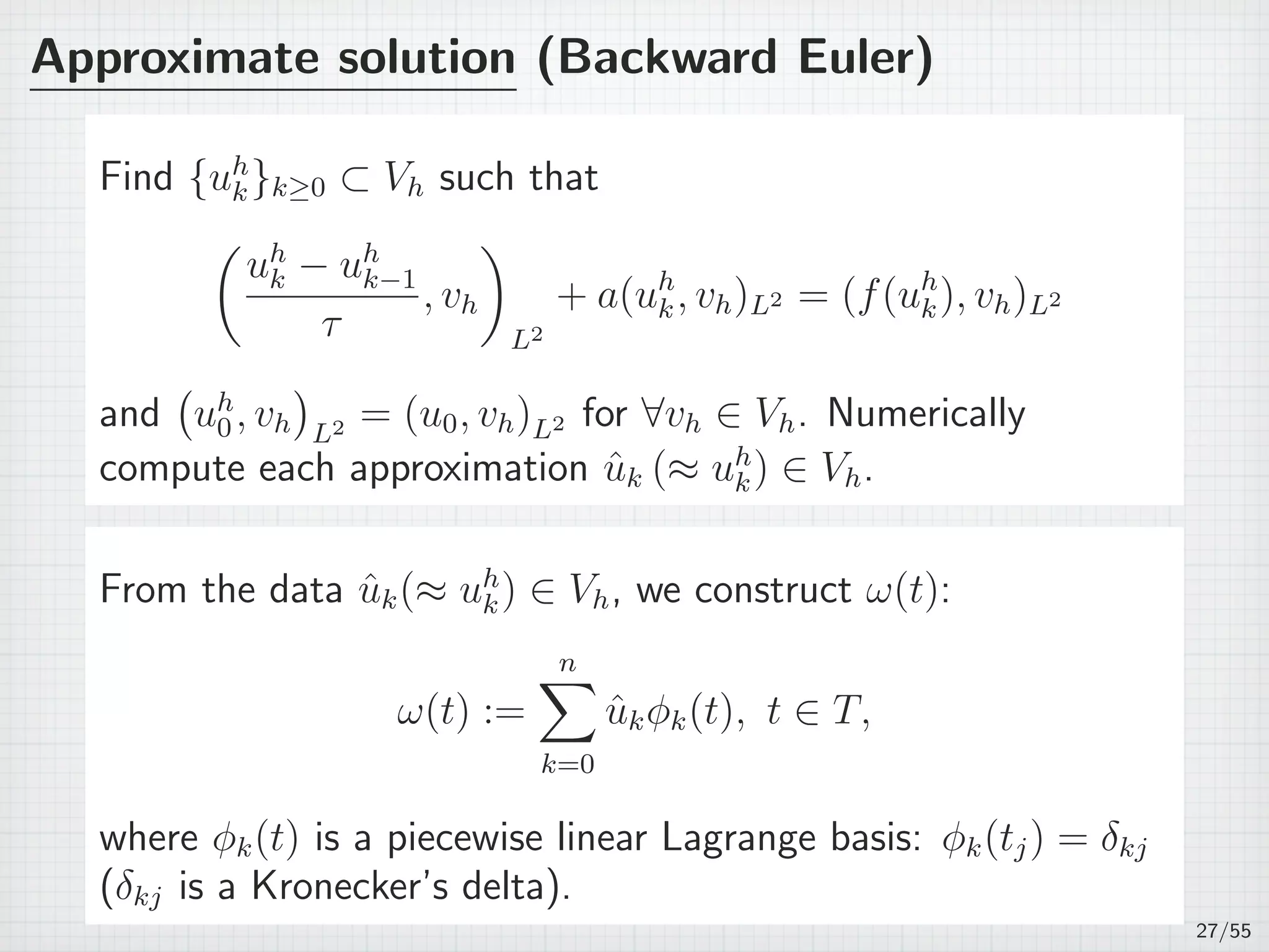
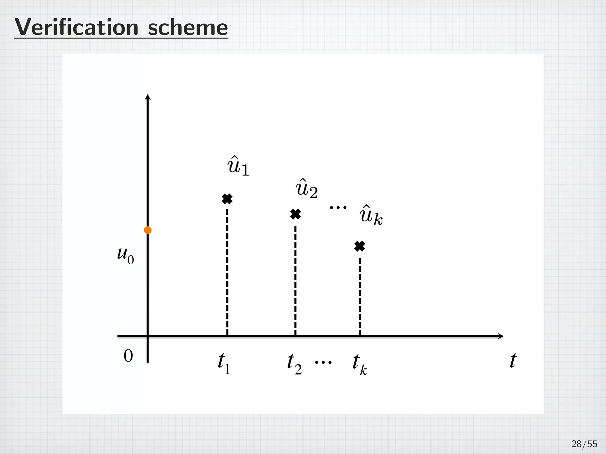
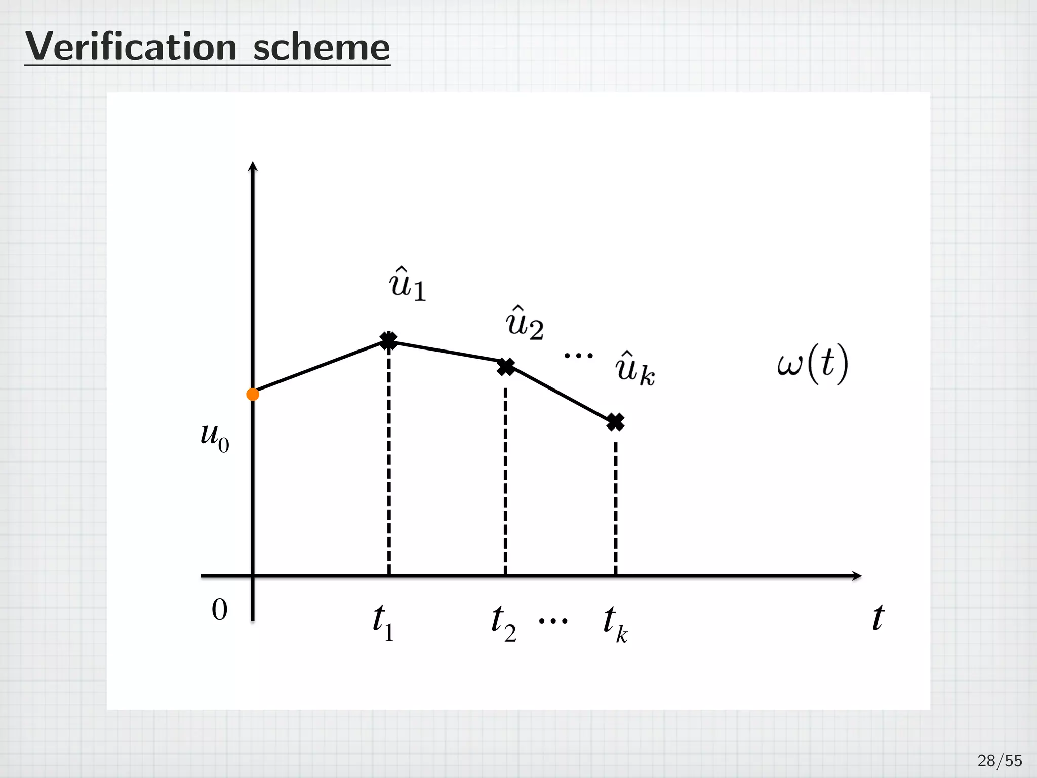
Starts from: ˆu0, ˆu1 ∈ Vh
ω(t) = ˆu0ϕ0(t) + ˆu1ϕ1(t), t ∈ J,
where ϕk(t) is a piecewise linear Lagrange basis: ϕk(tj) = δkj
(δkj is a Kronecker’s delta).
14/55](https://image.slidesharecdn.com/akitoshitakayasu-160128011103/75/Akitoshi-Takayasu-16-2048.jpg)
![Considered problem
J := (t0, t1] : arbitrary time interval. τ := t1 − t0.
(PJ )
∂tu + Au = f(u) in J × Ω,
u(t, x) = 0 on J × ∂Ω,
u(t0, x) = u0(x) in Ω,
where u0 is an initial function in H1
0 (Ω).
Vh ⊂ H1
0 (Ω) : a finite dimensional subspace.
Starts from: ˆu0, ˆu1 ∈ Vh
ω(t) = ˆu0ϕ0(t) + ˆu1ϕ1(t), t ∈ J,
where ϕk(t) is a piecewise linear Lagrange basis: ϕk(tj) = δkj
(δkj is a Kronecker’s delta).
14/55](https://image.slidesharecdn.com/akitoshitakayasu-160128011103/75/Akitoshi-Takayasu-17-2048.jpg)


![Theorem
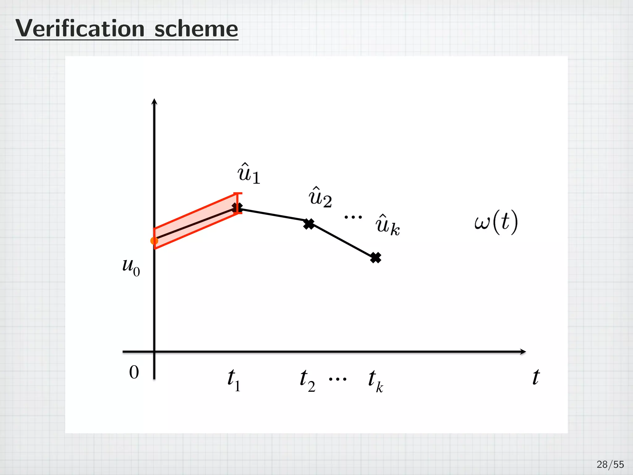
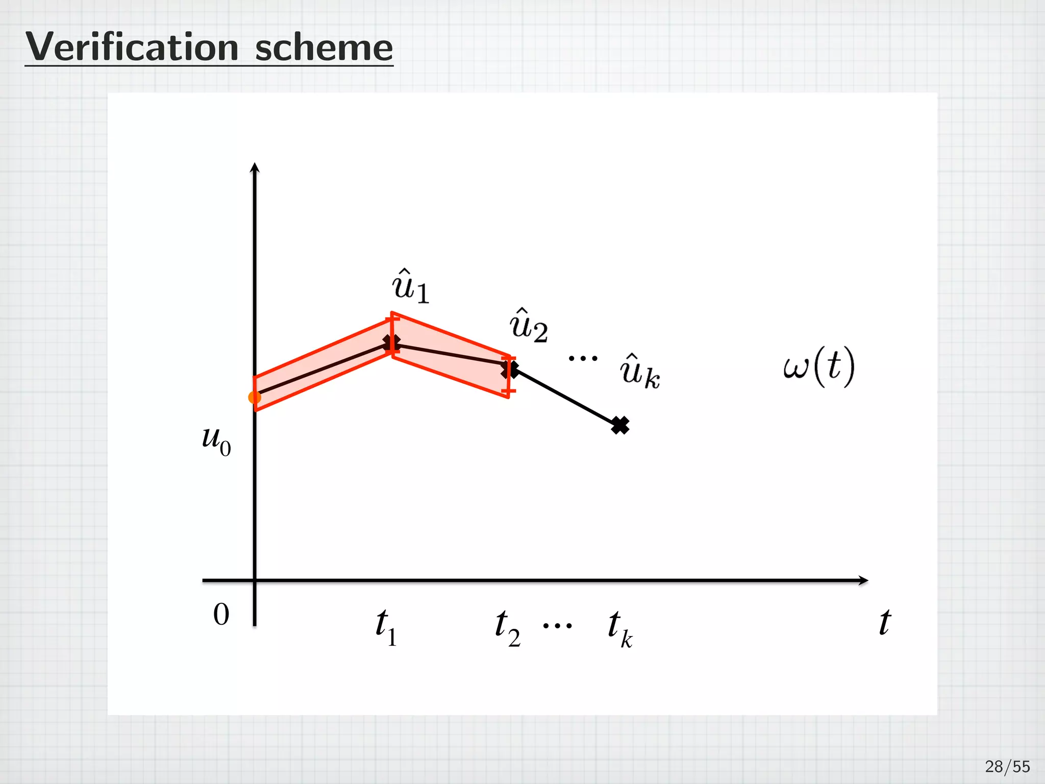
Assume that the initial function u0 satisfies ∥u0 − ˆu0∥H1
0
≤ ε0;
Assume that ω satisfies the following estimate:
∫ t
t0
e−(t−s)A
(∂tω(s) + Aω(s) − f(ω(s)))ds
L∞
(J;H1
0 (Ω))
≤ δ.
Assume that, for ∀ρ0 ∈ (0, ρ] with a certain ρ 0, f satisfies
∥f(φ) − f(ψ)∥L∞(J;L2(Ω)) ≤ Lρ0 ∥φ − ψ∥L∞
(J;H1
0 (Ω)),
where ∀φ, ψ ∈ BJ (ω, ρ0) ⊂ L∞
(J; H1
0 (Ω)). If
M
µ
ε0 +
2
µ
√
Mτ
e
Lρρ + δ ρ,
then the weak solution u(t), t ∈ J of (PJ ) uniquely exists in
the ball BJ (ω, ρ).
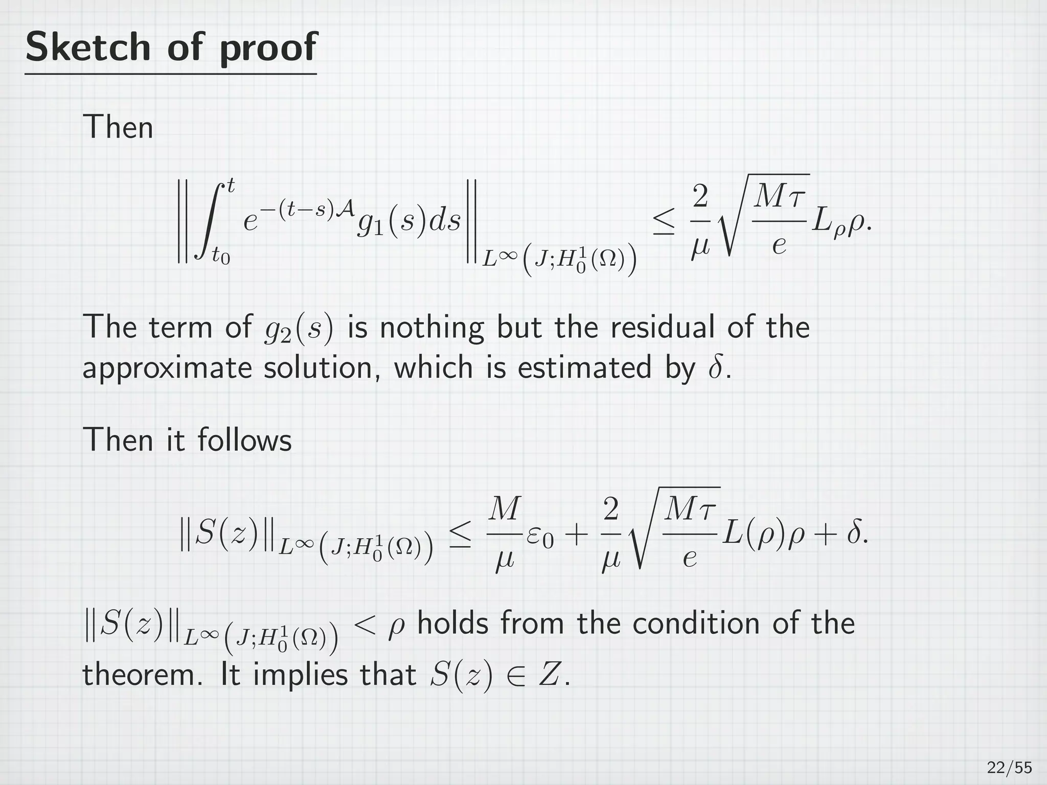
17/55](https://image.slidesharecdn.com/akitoshitakayasu-160128011103/75/Akitoshi-Takayasu-22-2048.jpg)
![Theorem
Assume that the initial function u0 satisfies ∥u0 − ˆu0∥H1
0
≤ ε0;
Assume that ω satisfies the following estimate:
∫ t
t0
e−(t−s)A
(∂tω(s) + Aω(s) − f(ω(s)))ds
L∞
(J;H1
0 (Ω))
≤ δ.
Assume that, for ∀ρ0 ∈ (0, ρ] with a certain ρ 0, f satisfies
∥f(φ) − f(ψ)∥L∞(J;L2(Ω)) ≤ Lρ0 ∥φ − ψ∥L∞
(J;H1
0 (Ω)),
where ∀φ, ψ ∈ BJ (ω, ρ0) ⊂ L∞
(J; H1
0 (Ω)). If
M
µ
ε0 +
2
µ
√
Mτ
e
Lρρ + δ ρ,
then the weak solution u(t), t ∈ J of (PJ ) uniquely exists in
the ball BJ (ω, ρ).
17/55](https://image.slidesharecdn.com/akitoshitakayasu-160128011103/75/Akitoshi-Takayasu-23-2048.jpg)
![Theorem
Assume that the initial function u0 satisfies ∥u0 − ˆu0∥H1
0
≤ ε0;
Assume that ω satisfies the following estimate:
∫ t
t0
e−(t−s)A
(∂tω(s) + Aω(s) − f(ω(s)))ds
L∞
(J;H1
0 (Ω))
≤ δ.
Assume that, for ∀ρ0 ∈ (0, ρ] with a certain ρ 0, f satisfies
∥f(φ) − f(ψ)∥L∞(J;L2(Ω)) ≤ Lρ0 ∥φ − ψ∥L∞
(J;H1
0 (Ω)),
where ∀φ, ψ ∈ BJ (ω, ρ0) ⊂ L∞
(J; H1
0 (Ω)). If
M
µ
ε0 +
2
µ
√
Mτ
e
Lρρ + δ ρ,
then the weak solution u(t), t ∈ J of (PJ ) uniquely exists in
the ball BJ (ω, ρ).
17/55](https://image.slidesharecdn.com/akitoshitakayasu-160128011103/75/Akitoshi-Takayasu-24-2048.jpg)
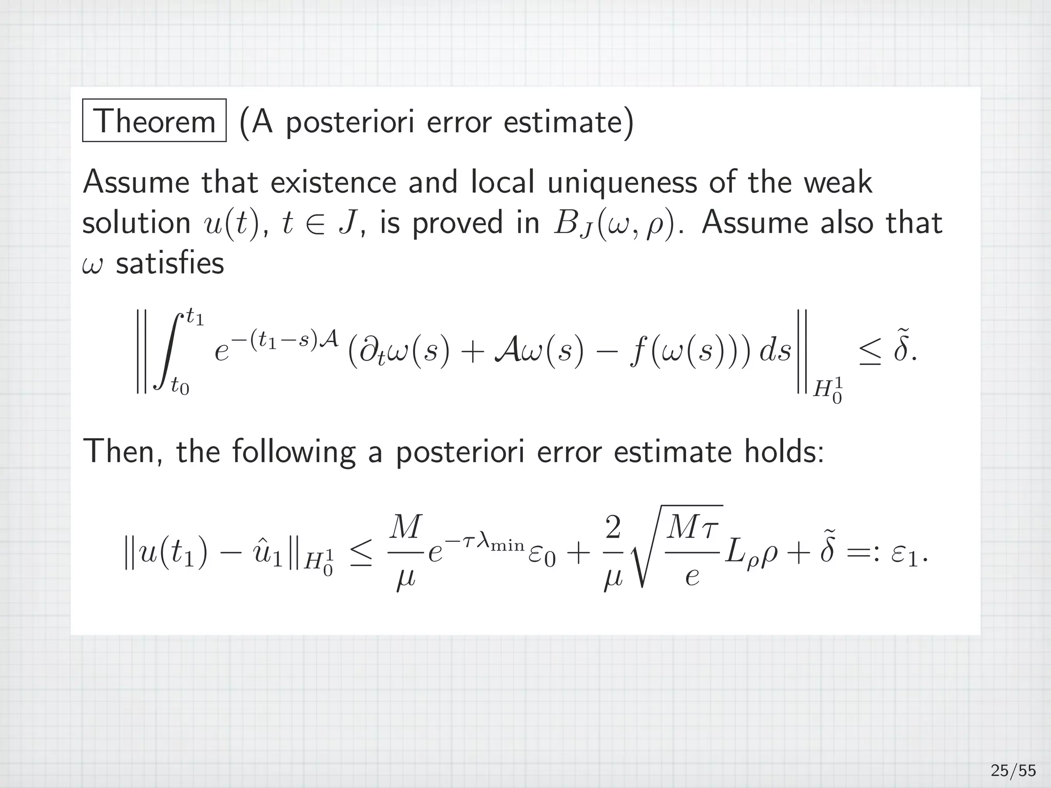
![Theorem
Assume that the initial function u0 satisfies ∥u0 − ˆu0∥H1
0
≤ ε0;
Assume that ω satisfies the following estimate:
∫ t
t0
e−(t−s)A
(∂tω(s) + Aω(s) − f(ω(s)))ds
L∞
(J;H1
0 (Ω))
≤ δ.
Assume that, for ∀ρ0 ∈ (0, ρ] with a certain ρ 0, f satisfies
∥f(φ) − f(ψ)∥L∞(J;L2(Ω)) ≤ Lρ0 ∥φ − ψ∥L∞
(J;H1
0 (Ω)),
where ∀φ, ψ ∈ BJ (ω, ρ0) ⊂ L∞
(J; H1
0 (Ω)). If
M
µ
ε0 +
2
µ
√
Mτ
e
Lρρ + δ ρ,
then the weak solution u(t), t ∈ J of (PJ ) uniquely exists in
the ball BJ (ω, ρ).
17/55](https://image.slidesharecdn.com/akitoshitakayasu-160128011103/75/Akitoshi-Takayasu-25-2048.jpg)
![Theorem
Assume that the initial function u0 satisfies ∥u0 − ˆu0∥H1
0
≤ ε0;
Assume that ω satisfies the following estimate:
∫ t
t0
e−(t−s)A
(∂tω(s) + Aω(s) − f(ω(s)))ds
L∞
(J;H1
0 (Ω))
≤ δ.
Assume that, for ∀ρ0 ∈ (0, ρ] with a certain ρ 0, f satisfies
∥f(φ) − f(ψ)∥L∞(J;L2(Ω)) ≤ Lρ0 ∥φ − ψ∥L∞
(J;H1
0 (Ω)),
where ∀φ, ψ ∈ BJ (ω, ρ0) ⊂ L∞
(J; H1
0 (Ω)). If
M
µ
ε0 +
2
µ
√
Mτ
e
Lρρ + δ ρ,
then the weak solution u(t), t ∈ J of (PJ ) uniquely exists in
the ball BJ (ω, ρ).
17/55](https://image.slidesharecdn.com/akitoshitakayasu-160128011103/75/Akitoshi-Takayasu-26-2048.jpg)

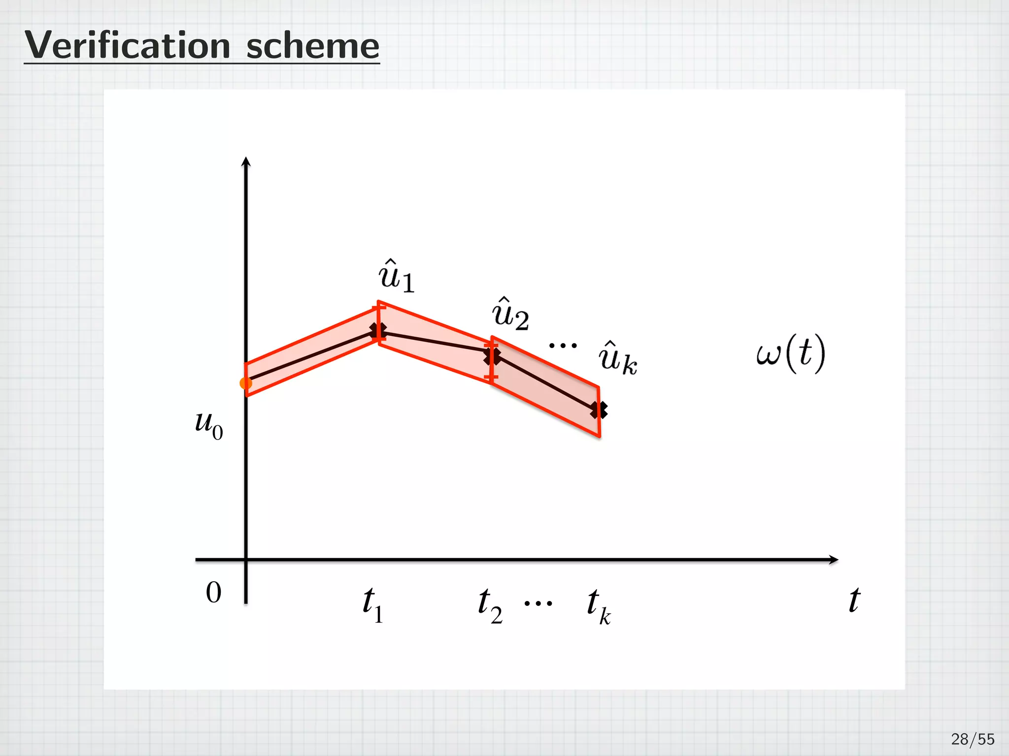
![On several intervals
For n ∈ N, 0 = t0 t1 · · · tn ∞.
Jk := (tk−1, tk], τk := tk − tk−1, and J =
∪
Jk. (k=1,2,...,n)
(PJ )
∂tu + Au = f(u) in J × Ω,
u(t, x) = 0 on J × ∂Ω,
u(0, x) = u0(x) in Ω,
where u0 ∈ H1
0 (Ω) is a given initial function satisfies
∥u0 − ˆu0∥H1
0
≤ ε0.
26/55](https://image.slidesharecdn.com/akitoshitakayasu-160128011103/75/Akitoshi-Takayasu-45-2048.jpg)

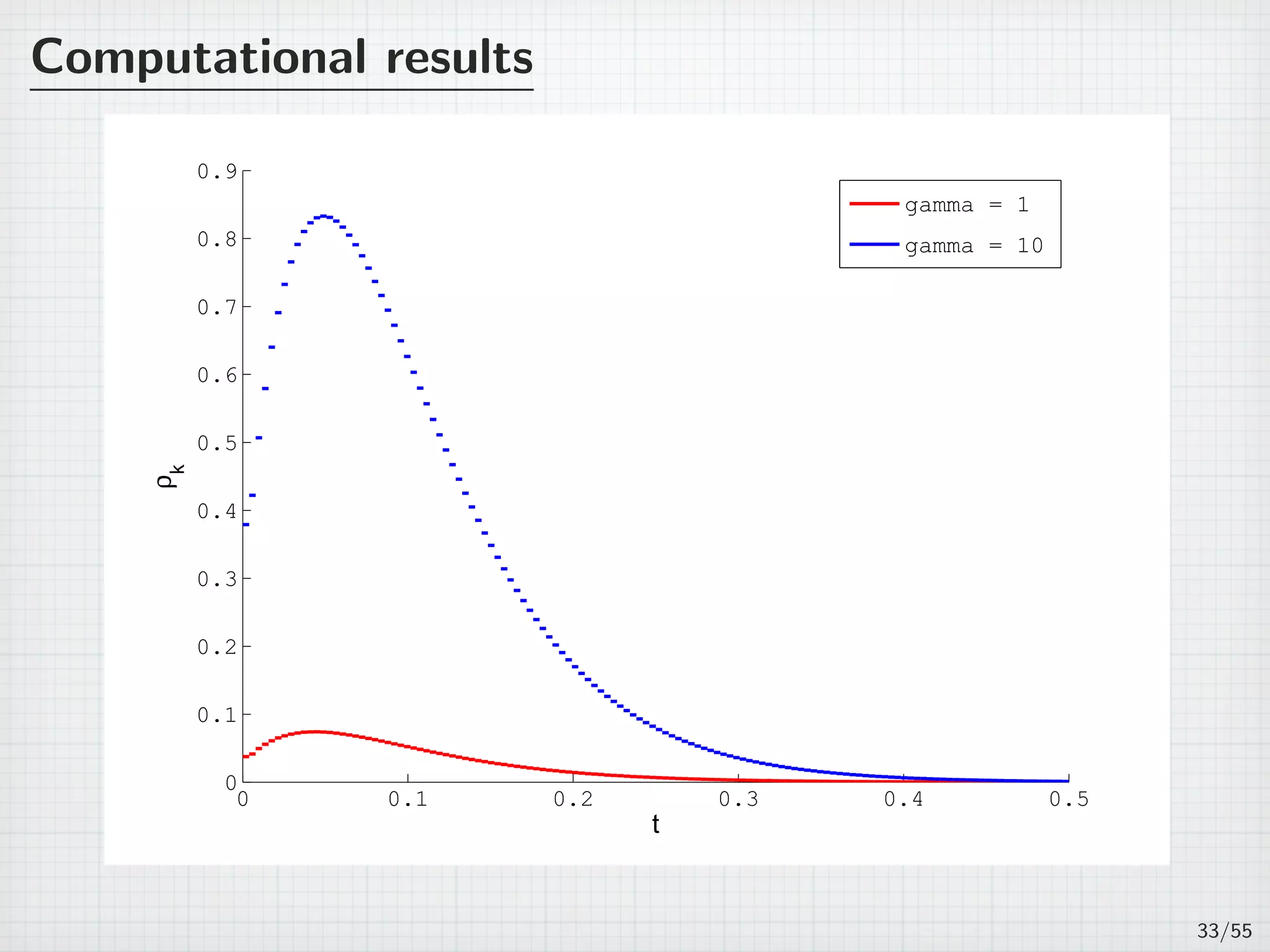
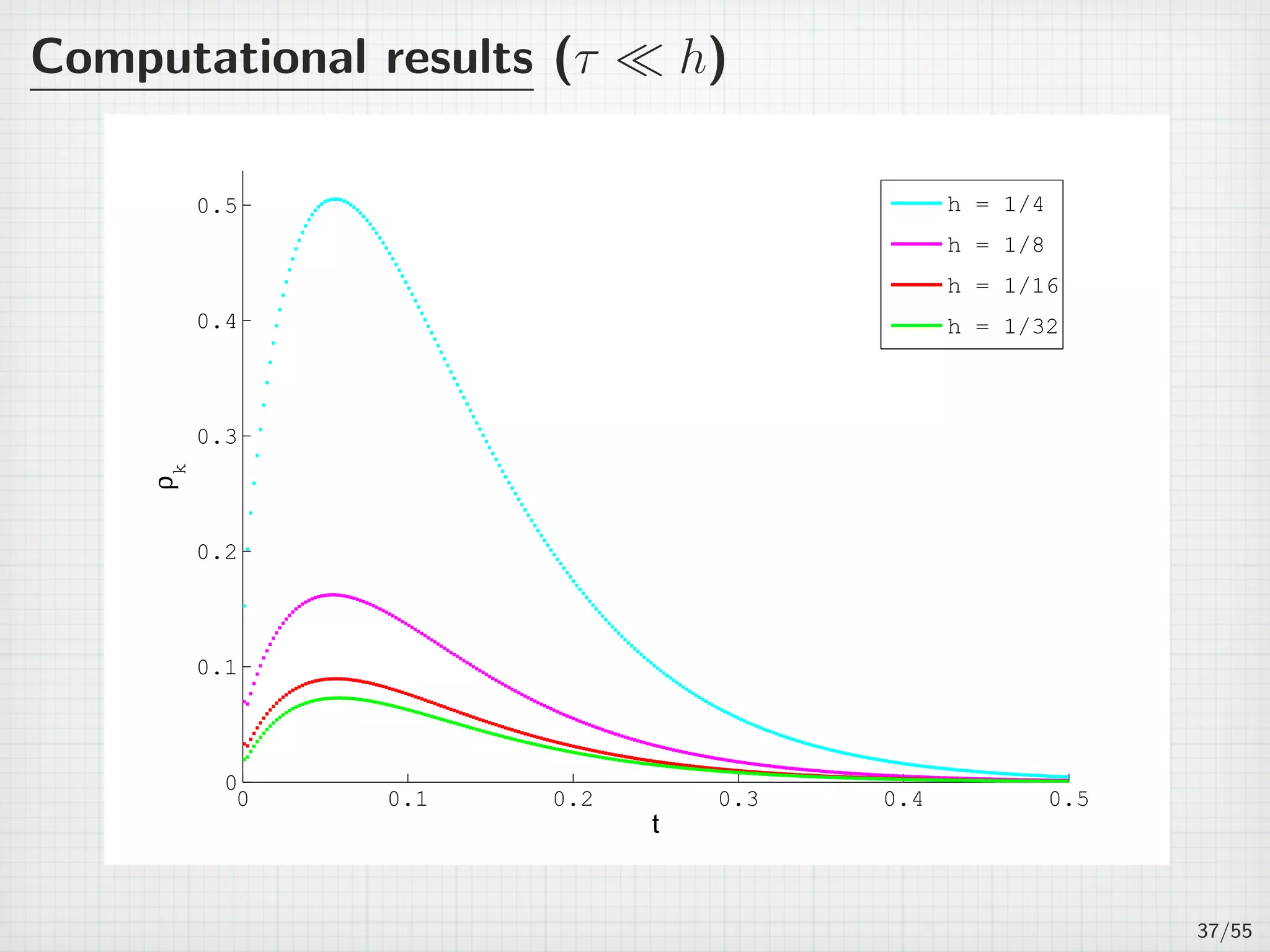
![Computational results
Table: h = 2−4
, τ = 2−8
, γ = 1.
Tk = (tk−1, tk] εk ρk
(0,0.0039062] 0.020155 0.037646
(0.0039062,0.0078125] 0.030051 0.041554
(0.0078125,0.011719] 0.038089 0.049313
(0.011719,0.015625] 0.044657 0.055699
(0.015625,0.019531] 0.050001 0.060873
...
...
...
(0.48047,0.48438] 0.00013041 0.00014184
(0.48438,0.48828] 0.00012186 0.00013255
(0.48828,0.49219] 0.00011388 0.00012386
(0.49219,0.49609] 0.00010641 0.00011573
(0.49609,0.5] 9.9431E-5 0.00010813
32/55](https://image.slidesharecdn.com/akitoshitakayasu-160128011103/75/Akitoshi-Takayasu-57-2048.jpg)

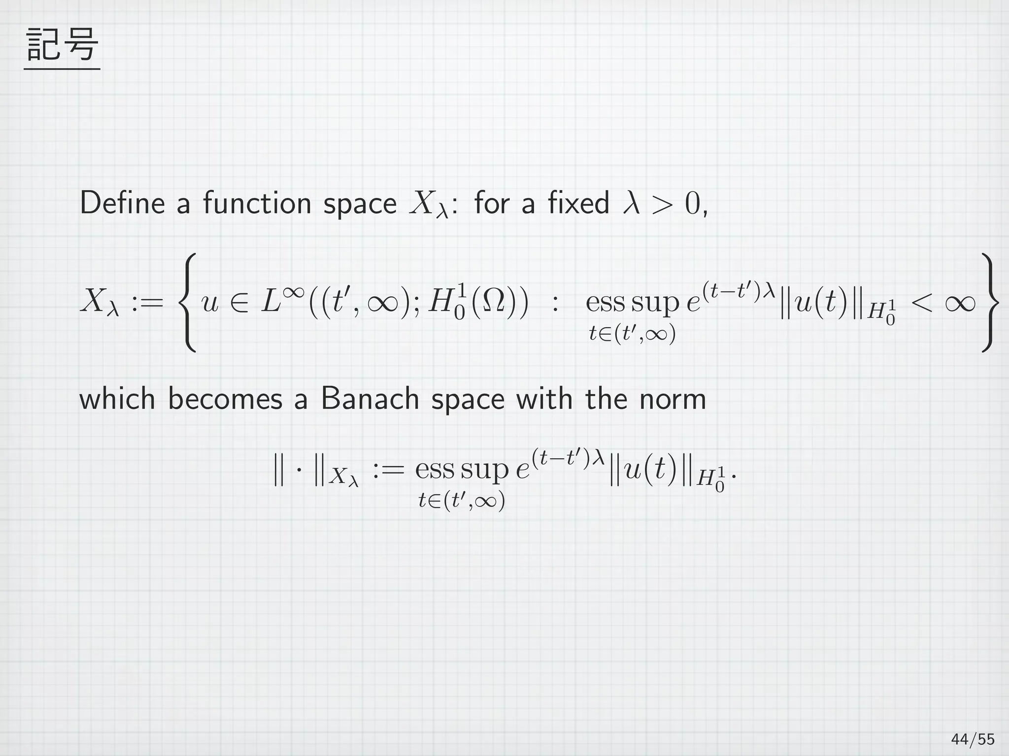
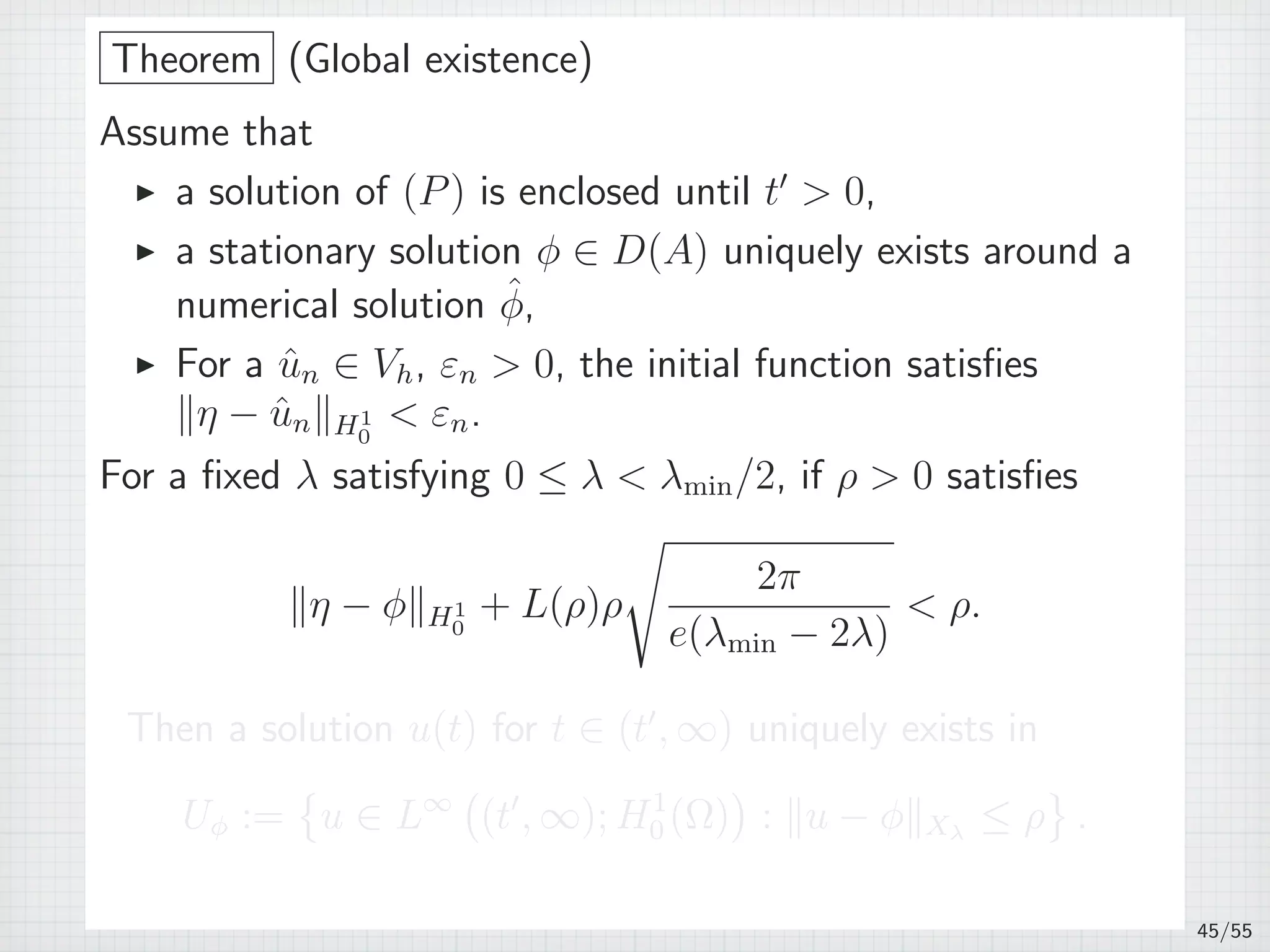
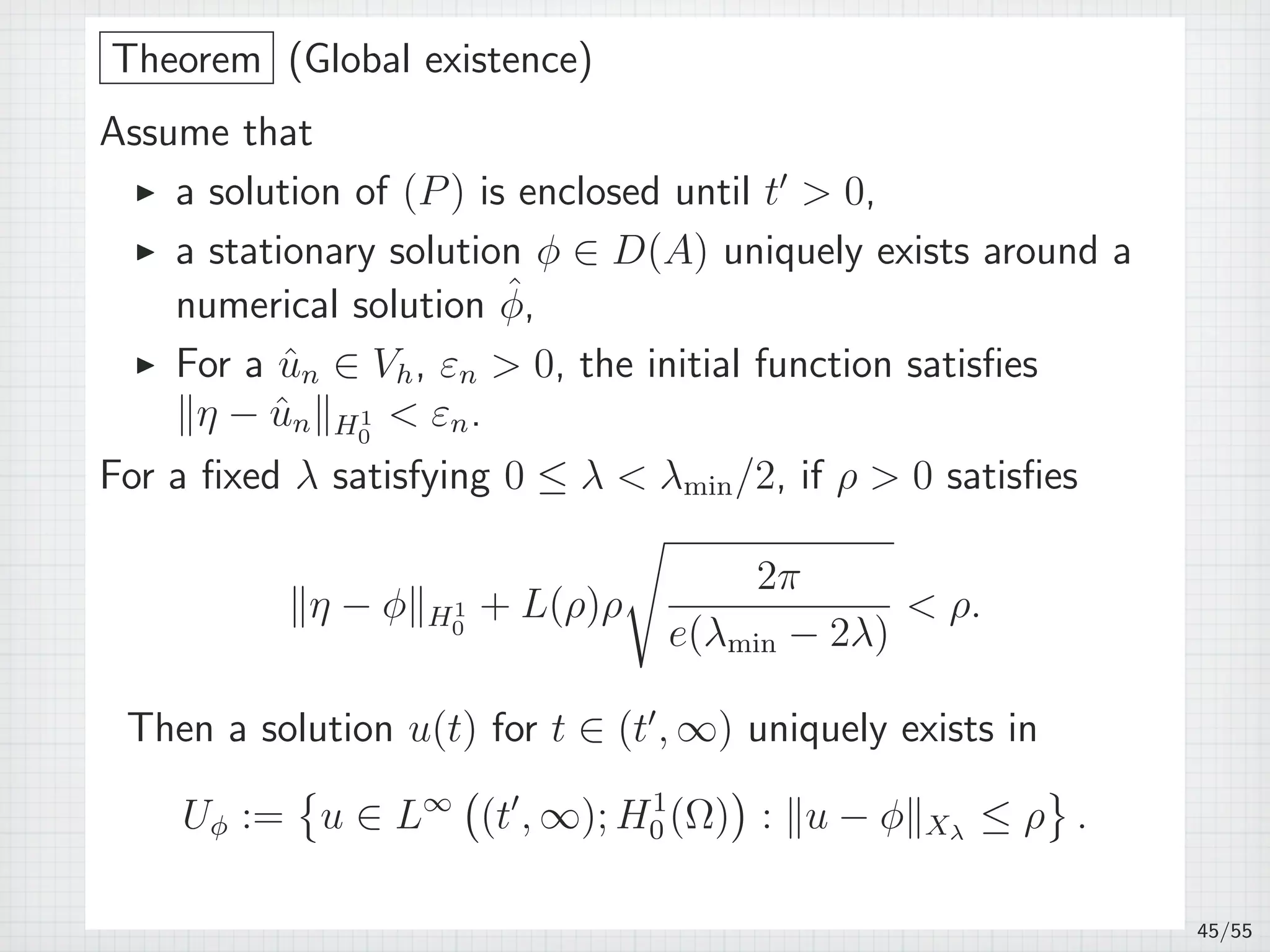
![記号
For ρ 0, v ∈ L∞
((t′
, ∞); H1
0 (Ω)), define a ball
B(v, ρ) :=
{
y ∈ L∞
(
(t′
, ∞); H1
0 (Ω)
)
: ∥y − v∥L∞
((t′,∞);H1
0 (Ω)) ≤ ρ
}
.
The Fr´echet derivative of f at w is denoted by
f′
[w] : L∞
((t′
, ∞); H1
0 (Ω)) → L∞
((t′
, ∞); L2
(Ω)).
For y ∈ B(v, ρ), we assume that there exists a non-decreasing
function L : R → R such that
∥f′
[y]u∥L∞(J;L2(Ω)) ≤ L(ρ)∥u∥H1
0
, u ∈ H1
0 (Ω).
43/55](https://image.slidesharecdn.com/akitoshitakayasu-160128011103/75/Akitoshi-Takayasu-71-2048.jpg)
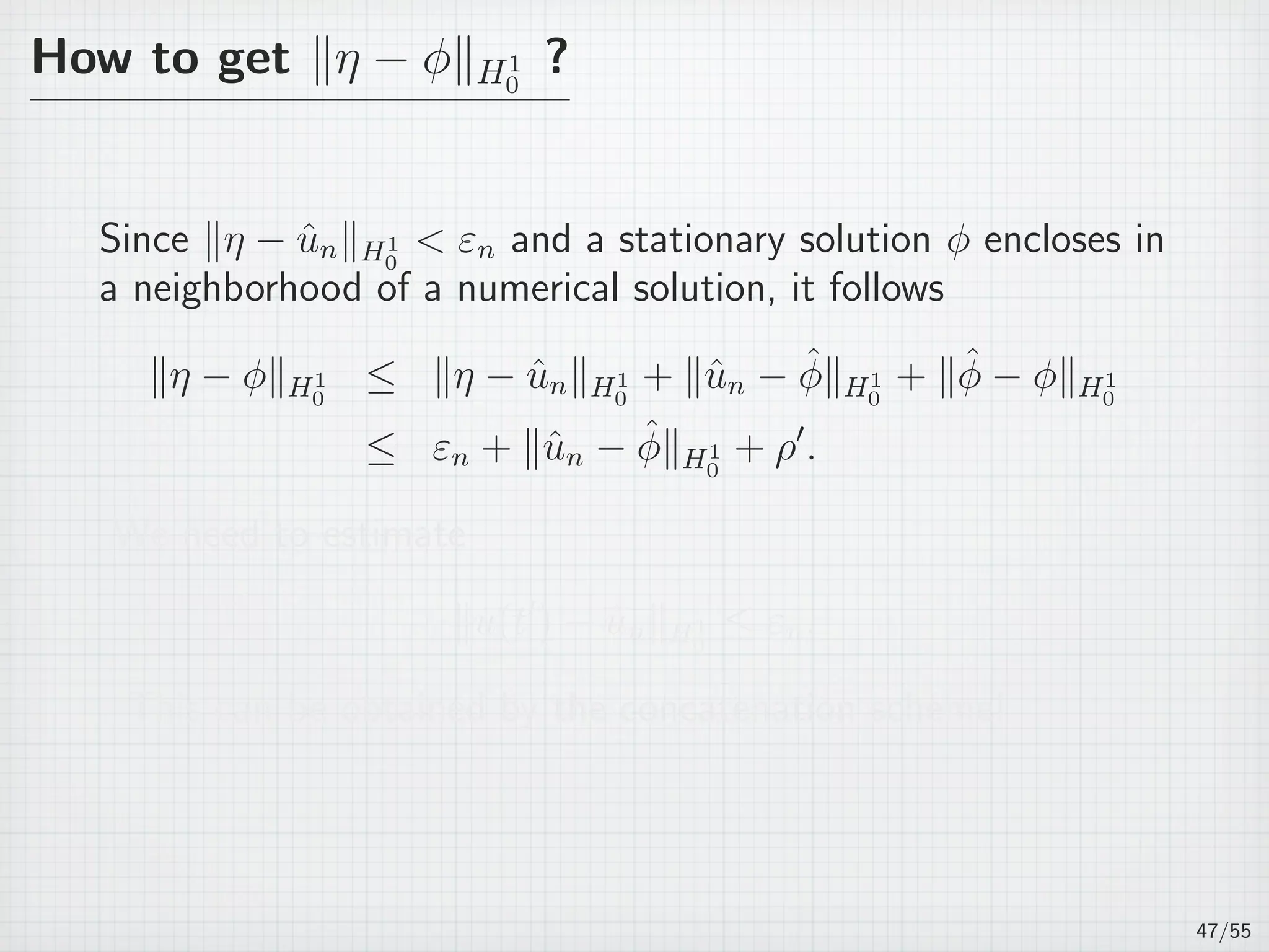
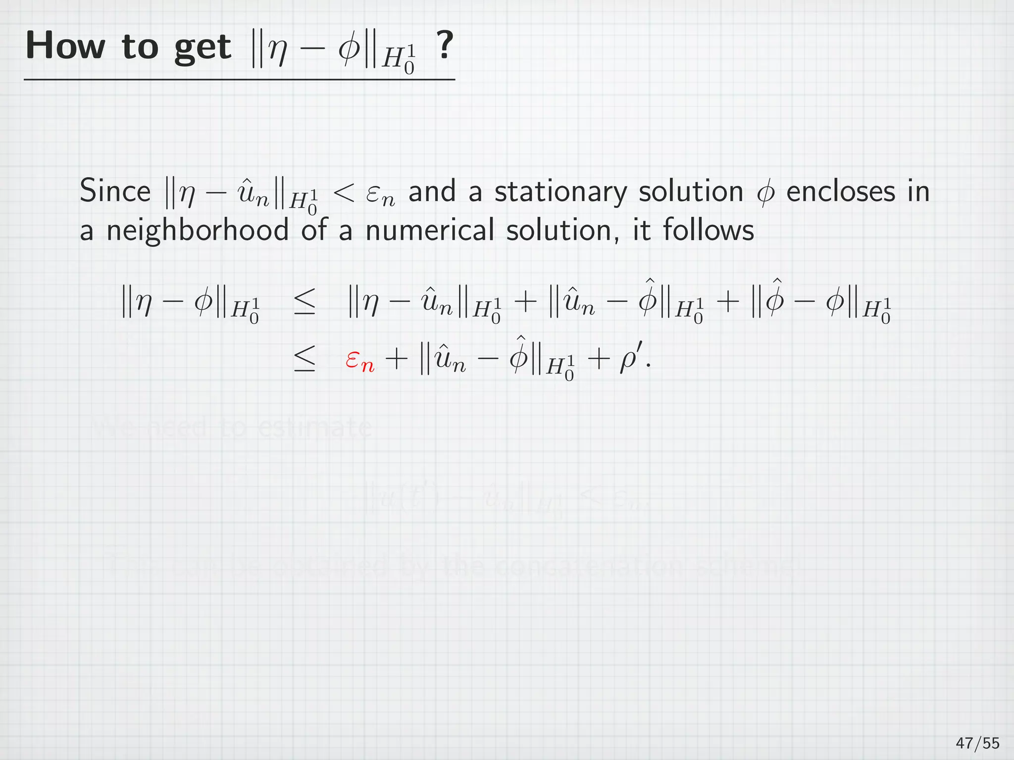
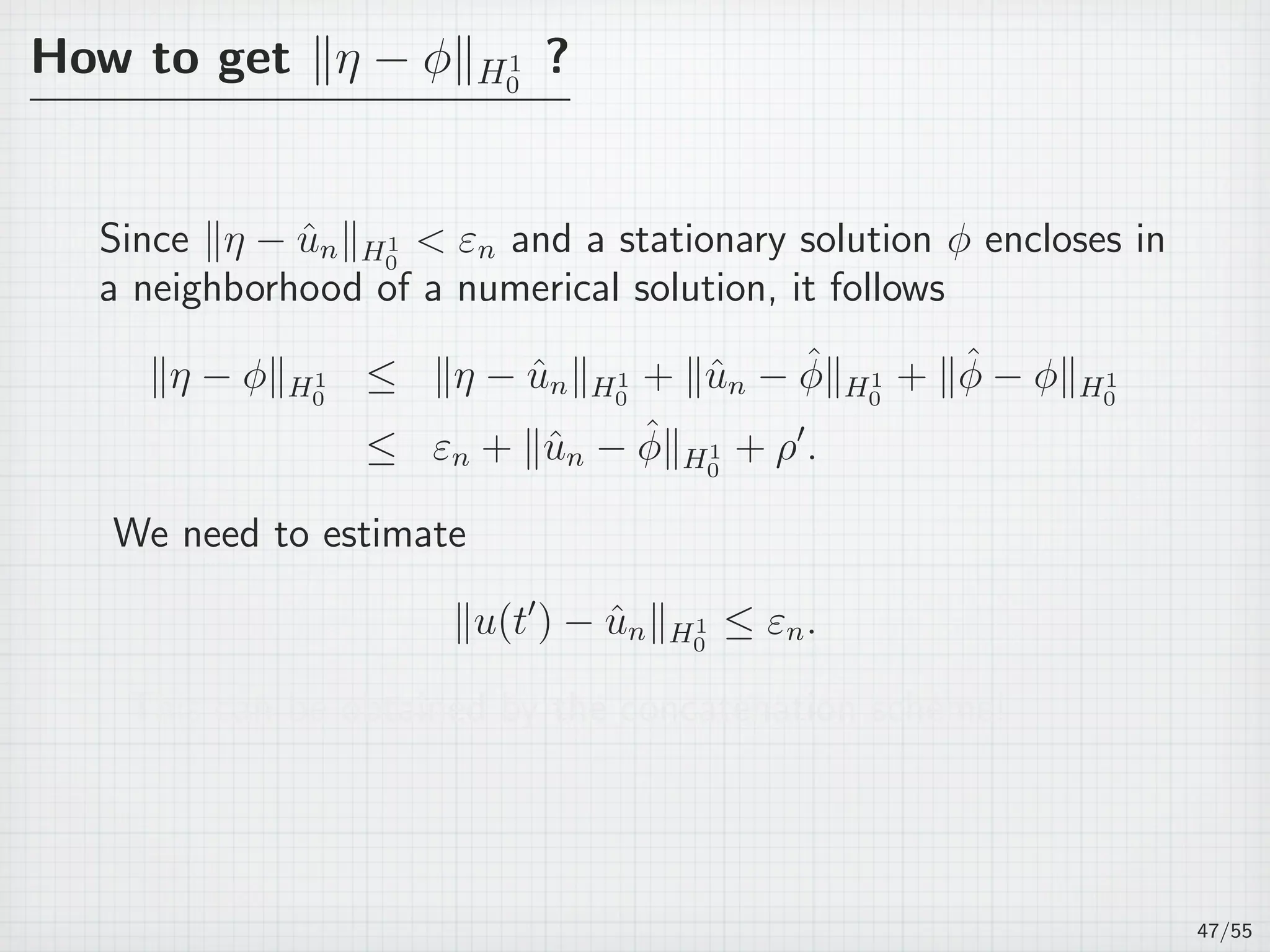
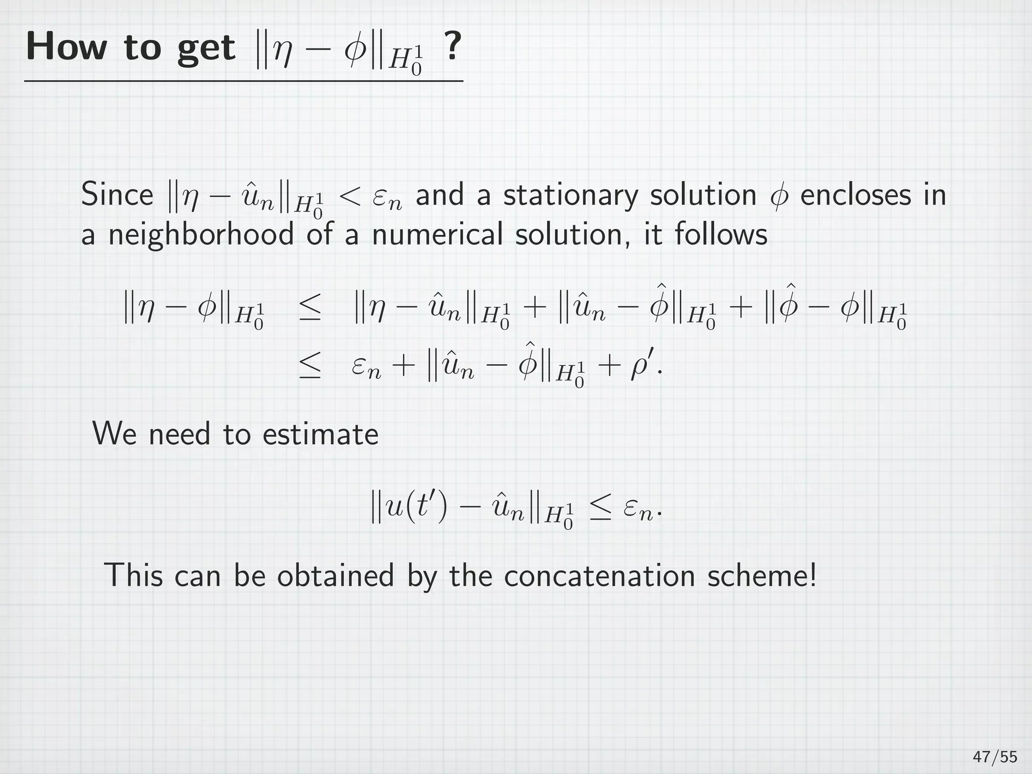
 − ψ2(s))∥L2 .
Since y ∈ Uϕ ⊂ B(ϕ, ρ) holds, we obtain
∥f(ψ1(s)) − f(ψ2(s))∥L2 ≤ L(ρ)∥ψ1(s) − ψ2(s)∥H1
0
.
46/55](https://image.slidesharecdn.com/akitoshitakayasu-160128011103/75/Akitoshi-Takayasu-78-2048.jpg)


![11.[104 111]analytical solution for telegraph equation by modified of sumudu ...](https://cdn.slidesharecdn.com/ss_thumbnails/11-104-111analyticalsolutionfortelegraphequationbymodifiedofsumudutransformelzakitransform-120513000219-phpapp01-thumbnail.jpg?width=640&height=640&fit=bounds)