Download to read offline


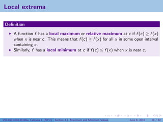
![The Extreme Value Theorem
Theorem (The Extreme Value Theorem)
Let f be a function which is continuous on the closed interval [a, b]. Then
f attains an absolute maximum value f (c) and an absolute minimum
value f (d) at numbers c and d in [a, b].
V63.0121.002.2010Su, Calculus I (NYU) Section 4.1 Maximum and Minimum Values June 8, 2010 12 / 32](https://image.slidesharecdn.com/lesson18-maximumandminimumvaluesslides-100610135316-phpapp01-121002231606-phpapp02/85/Lesson18-maximum_and_minimum_values_slides-16-320.jpg)
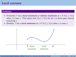
![The Extreme Value Theorem
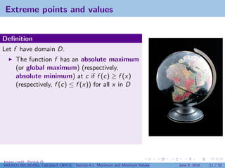
Theorem (The Extreme Value Theorem)
Let f be a function which is continuous on the closed interval [a, b]. Then
f attains an absolute maximum value f (c) and an absolute minimum
value f (d) at numbers c and d in [a, b].
a b
V63.0121.002.2010Su, Calculus I (NYU) Section 4.1 Maximum and Minimum Values June 8, 2010 12 / 32](https://image.slidesharecdn.com/lesson18-maximumandminimumvaluesslides-100610135316-phpapp01-121002231606-phpapp02/85/Lesson18-maximum_and_minimum_values_slides-17-320.jpg)
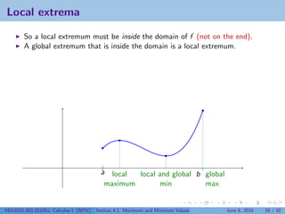
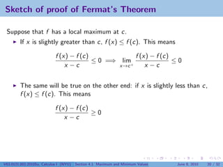
![The Extreme Value Theorem
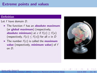
Theorem (The Extreme Value Theorem)
Let f be a function which is continuous on the closed interval [a, b]. Then
f attains an absolute maximum value f (c) and an absolute minimum
value f (d) at numbers c and d in [a, b].
maximum f (c)
value
minimum f (d)
value
a d c
b
minimum maximum
V63.0121.002.2010Su, Calculus I (NYU) Section 4.1 Maximum and Minimum Values June 8, 2010 12 / 32](https://image.slidesharecdn.com/lesson18-maximumandminimumvaluesslides-100610135316-phpapp01-121002231606-phpapp02/85/Lesson18-maximum_and_minimum_values_slides-18-320.jpg)
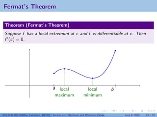
![Bad Example #1
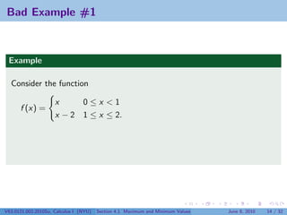
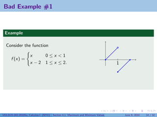
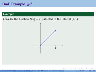
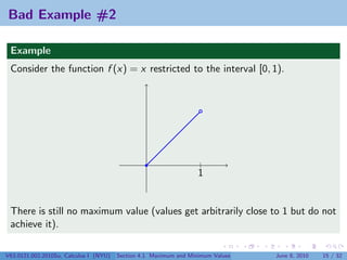
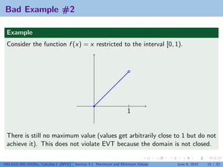
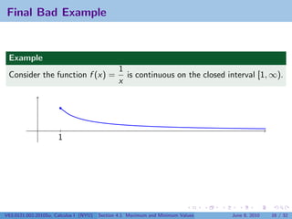
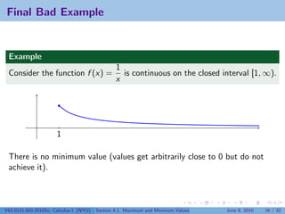
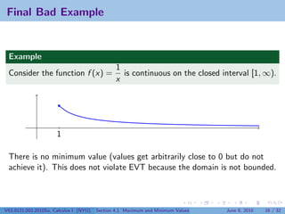
Example
Consider the function
x 0≤x <1
f (x) = |
x − 2 1 ≤ x ≤ 2. 1
Then although values of f (x) get arbitrarily close to 1 and never bigger
than 1, 1 is not the maximum value of f on [0, 1] because it is never
achieved.
V63.0121.002.2010Su, Calculus I (NYU) Section 4.1 Maximum and Minimum Values June 8, 2010 14 / 32](https://image.slidesharecdn.com/lesson18-maximumandminimumvaluesslides-100610135316-phpapp01-121002231606-phpapp02/85/Lesson18-maximum_and_minimum_values_slides-22-320.jpg)
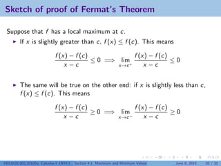
![Bad Example #1
Example
Consider the function
x 0≤x <1
f (x) = |
x − 2 1 ≤ x ≤ 2. 1
Then although values of f (x) get arbitrarily close to 1 and never bigger
than 1, 1 is not the maximum value of f on [0, 1] because it is never
achieved. This does not violate EVT because f is not continuous.
V63.0121.002.2010Su, Calculus I (NYU) Section 4.1 Maximum and Minimum Values June 8, 2010 14 / 32](https://image.slidesharecdn.com/lesson18-maximumandminimumvaluesslides-100610135316-phpapp01-121002231606-phpapp02/85/Lesson18-maximum_and_minimum_values_slides-23-320.jpg)
![Flowchart for placing extrema
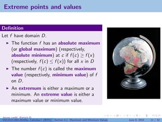
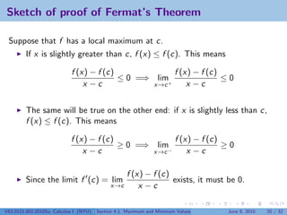
Thanks to Fermat
Suppose f is a continuous function on the closed, bounded interval [a, b],
and c is a global maximum point.
c is a
start
local max
Is f
Is c an f is not
no diff’ble at no
endpoint? diff at c
c?
yes yes
c = a or
f (c) = 0
c = b
V63.0121.002.2010Su, Calculus I (NYU) Section 4.1 Maximum and Minimum Values June 8, 2010 24 / 32](https://image.slidesharecdn.com/lesson18-maximumandminimumvaluesslides-100610135316-phpapp01-121002231606-phpapp02/85/Lesson18-maximum_and_minimum_values_slides-50-320.jpg)
![The Closed Interval Method
This means to find the maximum value of f on [a, b], we need to:
Evaluate f at the endpoints a and b
Evaluate f at the critical points or critical numbers x where either
f (x) = 0 or f is not differentiable at x.
The points with the largest function value are the global maximum
points
The points with the smallest or most negative function value are the
global minimum points.
V63.0121.002.2010Su, Calculus I (NYU) Section 4.1 Maximum and Minimum Values June 8, 2010 25 / 32](https://image.slidesharecdn.com/lesson18-maximumandminimumvaluesslides-100610135316-phpapp01-121002231606-phpapp02/85/Lesson18-maximum_and_minimum_values_slides-51-320.jpg)
![Extreme values of a linear function
Example
Find the extreme values of f (x) = 2x − 5 on [−1, 2].
V63.0121.002.2010Su, Calculus I (NYU) Section 4.1 Maximum and Minimum Values June 8, 2010 27 / 32](https://image.slidesharecdn.com/lesson18-maximumandminimumvaluesslides-100610135316-phpapp01-121002231606-phpapp02/85/Lesson18-maximum_and_minimum_values_slides-53-320.jpg)
![Extreme values of a linear function
Example
Find the extreme values of f (x) = 2x − 5 on [−1, 2].
Solution
Since f (x) = 2, which is never zero, we have no critical points and we
need only investigate the endpoints:
f (−1) = 2(−1) − 5 = −7
f (2) = 2(2) − 5 = −1
V63.0121.002.2010Su, Calculus I (NYU) Section 4.1 Maximum and Minimum Values June 8, 2010 27 / 32](https://image.slidesharecdn.com/lesson18-maximumandminimumvaluesslides-100610135316-phpapp01-121002231606-phpapp02/85/Lesson18-maximum_and_minimum_values_slides-54-320.jpg)
![Extreme values of a linear function
Example
Find the extreme values of f (x) = 2x − 5 on [−1, 2].
Solution
Since f (x) = 2, which is never zero, we have no critical points and we
need only investigate the endpoints:
f (−1) = 2(−1) − 5 = −7
f (2) = 2(2) − 5 = −1
So
The absolute minimum (point) is at −1; the minimum value is −7.
The absolute maximum (point) is at 2; the maximum value is −1.
V63.0121.002.2010Su, Calculus I (NYU) Section 4.1 Maximum and Minimum Values June 8, 2010 27 / 32](https://image.slidesharecdn.com/lesson18-maximumandminimumvaluesslides-100610135316-phpapp01-121002231606-phpapp02/85/Lesson18-maximum_and_minimum_values_slides-55-320.jpg)
![Extreme values of a quadratic function
Example
Find the extreme values of f (x) = x 2 − 1 on [−1, 2].
V63.0121.002.2010Su, Calculus I (NYU) Section 4.1 Maximum and Minimum Values June 8, 2010 28 / 32](https://image.slidesharecdn.com/lesson18-maximumandminimumvaluesslides-100610135316-phpapp01-121002231606-phpapp02/85/Lesson18-maximum_and_minimum_values_slides-56-320.jpg)
![Extreme values of a quadratic function
Example
Find the extreme values of f (x) = x 2 − 1 on [−1, 2].
Solution
We have f (x) = 2x, which is zero when x = 0.
V63.0121.002.2010Su, Calculus I (NYU) Section 4.1 Maximum and Minimum Values June 8, 2010 28 / 32](https://image.slidesharecdn.com/lesson18-maximumandminimumvaluesslides-100610135316-phpapp01-121002231606-phpapp02/85/Lesson18-maximum_and_minimum_values_slides-57-320.jpg)
![Extreme values of a quadratic function
Example
Find the extreme values of f (x) = x 2 − 1 on [−1, 2].
Solution
We have f (x) = 2x, which is zero when x = 0. So our points to check
are:
f (−1) =
f (0) =
f (2) =
V63.0121.002.2010Su, Calculus I (NYU) Section 4.1 Maximum and Minimum Values June 8, 2010 28 / 32](https://image.slidesharecdn.com/lesson18-maximumandminimumvaluesslides-100610135316-phpapp01-121002231606-phpapp02/85/Lesson18-maximum_and_minimum_values_slides-58-320.jpg)
![Extreme values of a quadratic function
Example
Find the extreme values of f (x) = x 2 − 1 on [−1, 2].
Solution
We have f (x) = 2x, which is zero when x = 0. So our points to check
are:
f (−1) = 0
f (0) =
f (2) =
V63.0121.002.2010Su, Calculus I (NYU) Section 4.1 Maximum and Minimum Values June 8, 2010 28 / 32](https://image.slidesharecdn.com/lesson18-maximumandminimumvaluesslides-100610135316-phpapp01-121002231606-phpapp02/85/Lesson18-maximum_and_minimum_values_slides-59-320.jpg)
![Extreme values of a quadratic function
Example
Find the extreme values of f (x) = x 2 − 1 on [−1, 2].
Solution
We have f (x) = 2x, which is zero when x = 0. So our points to check
are:
f (−1) = 0
f (0) = − 1
f (2) =
V63.0121.002.2010Su, Calculus I (NYU) Section 4.1 Maximum and Minimum Values June 8, 2010 28 / 32](https://image.slidesharecdn.com/lesson18-maximumandminimumvaluesslides-100610135316-phpapp01-121002231606-phpapp02/85/Lesson18-maximum_and_minimum_values_slides-60-320.jpg)
![Extreme values of a quadratic function
Example
Find the extreme values of f (x) = x 2 − 1 on [−1, 2].
Solution
We have f (x) = 2x, which is zero when x = 0. So our points to check
are:
f (−1) = 0
f (0) = − 1
f (2) = 3
V63.0121.002.2010Su, Calculus I (NYU) Section 4.1 Maximum and Minimum Values June 8, 2010 28 / 32](https://image.slidesharecdn.com/lesson18-maximumandminimumvaluesslides-100610135316-phpapp01-121002231606-phpapp02/85/Lesson18-maximum_and_minimum_values_slides-61-320.jpg)
![Extreme values of a quadratic function
Example
Find the extreme values of f (x) = x 2 − 1 on [−1, 2].
Solution
We have f (x) = 2x, which is zero when x = 0. So our points to check
are:
f (−1) = 0
f (0) = − 1 (absolute min)
f (2) = 3
V63.0121.002.2010Su, Calculus I (NYU) Section 4.1 Maximum and Minimum Values June 8, 2010 28 / 32](https://image.slidesharecdn.com/lesson18-maximumandminimumvaluesslides-100610135316-phpapp01-121002231606-phpapp02/85/Lesson18-maximum_and_minimum_values_slides-62-320.jpg)
![Extreme values of a quadratic function
Example
Find the extreme values of f (x) = x 2 − 1 on [−1, 2].
Solution
We have f (x) = 2x, which is zero when x = 0. So our points to check
are:
f (−1) = 0
f (0) = − 1 (absolute min)
f (2) = 3 (absolute max)
V63.0121.002.2010Su, Calculus I (NYU) Section 4.1 Maximum and Minimum Values June 8, 2010 28 / 32](https://image.slidesharecdn.com/lesson18-maximumandminimumvaluesslides-100610135316-phpapp01-121002231606-phpapp02/85/Lesson18-maximum_and_minimum_values_slides-63-320.jpg)
![Extreme values of a cubic function
Example
Find the extreme values of f (x) = 2x 3 − 3x 2 + 1 on [−1, 2].
V63.0121.002.2010Su, Calculus I (NYU) Section 4.1 Maximum and Minimum Values June 8, 2010 29 / 32](https://image.slidesharecdn.com/lesson18-maximumandminimumvaluesslides-100610135316-phpapp01-121002231606-phpapp02/85/Lesson18-maximum_and_minimum_values_slides-64-320.jpg)
![Extreme values of a cubic function
Example
Find the extreme values of f (x) = 2x 3 − 3x 2 + 1 on [−1, 2].
Solution
Since f (x) = 6x 2 − 6x = 6x(x − 1), we have critical points at x = 0 and
x = 1.
V63.0121.002.2010Su, Calculus I (NYU) Section 4.1 Maximum and Minimum Values June 8, 2010 29 / 32](https://image.slidesharecdn.com/lesson18-maximumandminimumvaluesslides-100610135316-phpapp01-121002231606-phpapp02/85/Lesson18-maximum_and_minimum_values_slides-65-320.jpg)
![Extreme values of a cubic function
Example
Find the extreme values of f (x) = 2x 3 − 3x 2 + 1 on [−1, 2].
Solution
Since f (x) = 6x 2 − 6x = 6x(x − 1), we have critical points at x = 0 and
x = 1. The values to check are
f (−1) =
f (0) =
f (1) =
f (2) =
V63.0121.002.2010Su, Calculus I (NYU) Section 4.1 Maximum and Minimum Values June 8, 2010 29 / 32](https://image.slidesharecdn.com/lesson18-maximumandminimumvaluesslides-100610135316-phpapp01-121002231606-phpapp02/85/Lesson18-maximum_and_minimum_values_slides-66-320.jpg)
![Extreme values of a cubic function
Example
Find the extreme values of f (x) = 2x 3 − 3x 2 + 1 on [−1, 2].
Solution
Since f (x) = 6x 2 − 6x = 6x(x − 1), we have critical points at x = 0 and
x = 1. The values to check are
f (−1) = − 4
f (0) =
f (1) =
f (2) =
V63.0121.002.2010Su, Calculus I (NYU) Section 4.1 Maximum and Minimum Values June 8, 2010 29 / 32](https://image.slidesharecdn.com/lesson18-maximumandminimumvaluesslides-100610135316-phpapp01-121002231606-phpapp02/85/Lesson18-maximum_and_minimum_values_slides-67-320.jpg)
![Extreme values of a cubic function
Example
Find the extreme values of f (x) = 2x 3 − 3x 2 + 1 on [−1, 2].
Solution
Since f (x) = 6x 2 − 6x = 6x(x − 1), we have critical points at x = 0 and
x = 1. The values to check are
f (−1) = − 4
f (0) = 1
f (1) =
f (2) =
V63.0121.002.2010Su, Calculus I (NYU) Section 4.1 Maximum and Minimum Values June 8, 2010 29 / 32](https://image.slidesharecdn.com/lesson18-maximumandminimumvaluesslides-100610135316-phpapp01-121002231606-phpapp02/85/Lesson18-maximum_and_minimum_values_slides-68-320.jpg)
![Extreme values of a cubic function
Example
Find the extreme values of f (x) = 2x 3 − 3x 2 + 1 on [−1, 2].
Solution
Since f (x) = 6x 2 − 6x = 6x(x − 1), we have critical points at x = 0 and
x = 1. The values to check are
f (−1) = − 4
f (0) = 1
f (1) = 0
f (2) =
V63.0121.002.2010Su, Calculus I (NYU) Section 4.1 Maximum and Minimum Values June 8, 2010 29 / 32](https://image.slidesharecdn.com/lesson18-maximumandminimumvaluesslides-100610135316-phpapp01-121002231606-phpapp02/85/Lesson18-maximum_and_minimum_values_slides-69-320.jpg)
![Extreme values of a cubic function
Example
Find the extreme values of f (x) = 2x 3 − 3x 2 + 1 on [−1, 2].
Solution
Since f (x) = 6x 2 − 6x = 6x(x − 1), we have critical points at x = 0 and
x = 1. The values to check are
f (−1) = − 4
f (0) = 1
f (1) = 0
f (2) = 5
V63.0121.002.2010Su, Calculus I (NYU) Section 4.1 Maximum and Minimum Values June 8, 2010 29 / 32](https://image.slidesharecdn.com/lesson18-maximumandminimumvaluesslides-100610135316-phpapp01-121002231606-phpapp02/85/Lesson18-maximum_and_minimum_values_slides-70-320.jpg)
![Extreme values of a cubic function
Example
Find the extreme values of f (x) = 2x 3 − 3x 2 + 1 on [−1, 2].
Solution
Since f (x) = 6x 2 − 6x = 6x(x − 1), we have critical points at x = 0 and
x = 1. The values to check are
f (−1) = − 4 (global min)
f (0) = 1
f (1) = 0
f (2) = 5
V63.0121.002.2010Su, Calculus I (NYU) Section 4.1 Maximum and Minimum Values June 8, 2010 29 / 32](https://image.slidesharecdn.com/lesson18-maximumandminimumvaluesslides-100610135316-phpapp01-121002231606-phpapp02/85/Lesson18-maximum_and_minimum_values_slides-71-320.jpg)
![Extreme values of a cubic function
Example
Find the extreme values of f (x) = 2x 3 − 3x 2 + 1 on [−1, 2].
Solution
Since f (x) = 6x 2 − 6x = 6x(x − 1), we have critical points at x = 0 and
x = 1. The values to check are
f (−1) = − 4 (global min)
f (0) = 1
f (1) = 0
f (2) = 5 (global max)
V63.0121.002.2010Su, Calculus I (NYU) Section 4.1 Maximum and Minimum Values June 8, 2010 29 / 32](https://image.slidesharecdn.com/lesson18-maximumandminimumvaluesslides-100610135316-phpapp01-121002231606-phpapp02/85/Lesson18-maximum_and_minimum_values_slides-72-320.jpg)
![Extreme values of a cubic function
Example
Find the extreme values of f (x) = 2x 3 − 3x 2 + 1 on [−1, 2].
Solution
Since f (x) = 6x 2 − 6x = 6x(x − 1), we have critical points at x = 0 and
x = 1. The values to check are
f (−1) = − 4 (global min)
f (0) = 1 (local max)
f (1) = 0
f (2) = 5 (global max)
V63.0121.002.2010Su, Calculus I (NYU) Section 4.1 Maximum and Minimum Values June 8, 2010 29 / 32](https://image.slidesharecdn.com/lesson18-maximumandminimumvaluesslides-100610135316-phpapp01-121002231606-phpapp02/85/Lesson18-maximum_and_minimum_values_slides-73-320.jpg)
![Extreme values of a cubic function
Example
Find the extreme values of f (x) = 2x 3 − 3x 2 + 1 on [−1, 2].
Solution
Since f (x) = 6x 2 − 6x = 6x(x − 1), we have critical points at x = 0 and
x = 1. The values to check are
f (−1) = − 4 (global min)
f (0) = 1 (local max)
f (1) = 0 (local min)
f (2) = 5 (global max)
V63.0121.002.2010Su, Calculus I (NYU) Section 4.1 Maximum and Minimum Values June 8, 2010 29 / 32](https://image.slidesharecdn.com/lesson18-maximumandminimumvaluesslides-100610135316-phpapp01-121002231606-phpapp02/85/Lesson18-maximum_and_minimum_values_slides-74-320.jpg)
![Extreme values of an algebraic function
Example
Find the extreme values of f (x) = x 2/3 (x + 2) on [−1, 2].
V63.0121.002.2010Su, Calculus I (NYU) Section 4.1 Maximum and Minimum Values June 8, 2010 30 / 32](https://image.slidesharecdn.com/lesson18-maximumandminimumvaluesslides-100610135316-phpapp01-121002231606-phpapp02/85/Lesson18-maximum_and_minimum_values_slides-75-320.jpg)
![Extreme values of an algebraic function
Example
Find the extreme values of f (x) = x 2/3 (x + 2) on [−1, 2].
Solution
Write f (x) = x 5/3 + 2x 2/3 , then
5 4 1
f (x) = x 2/3 + x −1/3 = x −1/3 (5x + 4)
3 3 3
Thus f (−4/5) = 0 and f is not differentiable at 0.
V63.0121.002.2010Su, Calculus I (NYU) Section 4.1 Maximum and Minimum Values June 8, 2010 30 / 32](https://image.slidesharecdn.com/lesson18-maximumandminimumvaluesslides-100610135316-phpapp01-121002231606-phpapp02/85/Lesson18-maximum_and_minimum_values_slides-76-320.jpg)
![Extreme values of an algebraic function
Example
Find the extreme values of f (x) = x 2/3 (x + 2) on [−1, 2].
Solution
Write f (x) = x 5/3 + 2x 2/3 , then
5 4 1
f (x) = x 2/3 + x −1/3 = x −1/3 (5x + 4)
3 3 3
Thus f (−4/5) = 0 and f is not differentiable at 0. So our points to check
are:
f (−1) =
f (−4/5) =
f (0) =
f (2) =
V63.0121.002.2010Su, Calculus I (NYU) Section 4.1 Maximum and Minimum Values June 8, 2010 30 / 32](https://image.slidesharecdn.com/lesson18-maximumandminimumvaluesslides-100610135316-phpapp01-121002231606-phpapp02/85/Lesson18-maximum_and_minimum_values_slides-77-320.jpg)
![Extreme values of an algebraic function
Example
Find the extreme values of f (x) = x 2/3 (x + 2) on [−1, 2].
Solution
Write f (x) = x 5/3 + 2x 2/3 , then
5 4 1
f (x) = x 2/3 + x −1/3 = x −1/3 (5x + 4)
3 3 3
Thus f (−4/5) = 0 and f is not differentiable at 0. So our points to check
are:
f (−1) = 1
f (−4/5) =
f (0) =
f (2) =
V63.0121.002.2010Su, Calculus I (NYU) Section 4.1 Maximum and Minimum Values June 8, 2010 30 / 32](https://image.slidesharecdn.com/lesson18-maximumandminimumvaluesslides-100610135316-phpapp01-121002231606-phpapp02/85/Lesson18-maximum_and_minimum_values_slides-78-320.jpg)
![Extreme values of an algebraic function
Example
Find the extreme values of f (x) = x 2/3 (x + 2) on [−1, 2].
Solution
Write f (x) = x 5/3 + 2x 2/3 , then
5 4 1
f (x) = x 2/3 + x −1/3 = x −1/3 (5x + 4)
3 3 3
Thus f (−4/5) = 0 and f is not differentiable at 0. So our points to check
are:
f (−1) = 1
f (−4/5) = 1.0341
f (0) =
f (2) =
V63.0121.002.2010Su, Calculus I (NYU) Section 4.1 Maximum and Minimum Values June 8, 2010 30 / 32](https://image.slidesharecdn.com/lesson18-maximumandminimumvaluesslides-100610135316-phpapp01-121002231606-phpapp02/85/Lesson18-maximum_and_minimum_values_slides-79-320.jpg)
![Extreme values of an algebraic function
Example
Find the extreme values of f (x) = x 2/3 (x + 2) on [−1, 2].
Solution
Write f (x) = x 5/3 + 2x 2/3 , then
5 4 1
f (x) = x 2/3 + x −1/3 = x −1/3 (5x + 4)
3 3 3
Thus f (−4/5) = 0 and f is not differentiable at 0. So our points to check
are:
f (−1) = 1
f (−4/5) = 1.0341
f (0) = 0
f (2) =
V63.0121.002.2010Su, Calculus I (NYU) Section 4.1 Maximum and Minimum Values June 8, 2010 30 / 32](https://image.slidesharecdn.com/lesson18-maximumandminimumvaluesslides-100610135316-phpapp01-121002231606-phpapp02/85/Lesson18-maximum_and_minimum_values_slides-80-320.jpg)
![Extreme values of an algebraic function
Example
Find the extreme values of f (x) = x 2/3 (x + 2) on [−1, 2].
Solution
Write f (x) = x 5/3 + 2x 2/3 , then
5 4 1
f (x) = x 2/3 + x −1/3 = x −1/3 (5x + 4)
3 3 3
Thus f (−4/5) = 0 and f is not differentiable at 0. So our points to check
are:
f (−1) = 1
f (−4/5) = 1.0341
f (0) = 0
f (2) = 6.3496
V63.0121.002.2010Su, Calculus I (NYU) Section 4.1 Maximum and Minimum Values June 8, 2010 30 / 32](https://image.slidesharecdn.com/lesson18-maximumandminimumvaluesslides-100610135316-phpapp01-121002231606-phpapp02/85/Lesson18-maximum_and_minimum_values_slides-81-320.jpg)
![Extreme values of an algebraic function
Example
Find the extreme values of f (x) = x 2/3 (x + 2) on [−1, 2].
Solution
Write f (x) = x 5/3 + 2x 2/3 , then
5 4 1
f (x) = x 2/3 + x −1/3 = x −1/3 (5x + 4)
3 3 3
Thus f (−4/5) = 0 and f is not differentiable at 0. So our points to check
are:
f (−1) = 1
f (−4/5) = 1.0341
f (0) = 0 (absolute min)
f (2) = 6.3496
V63.0121.002.2010Su, Calculus I (NYU) Section 4.1 Maximum and Minimum Values June 8, 2010 30 / 32](https://image.slidesharecdn.com/lesson18-maximumandminimumvaluesslides-100610135316-phpapp01-121002231606-phpapp02/85/Lesson18-maximum_and_minimum_values_slides-82-320.jpg)
![Extreme values of an algebraic function
Example
Find the extreme values of f (x) = x 2/3 (x + 2) on [−1, 2].
Solution
Write f (x) = x 5/3 + 2x 2/3 , then
5 4 1
f (x) = x 2/3 + x −1/3 = x −1/3 (5x + 4)
3 3 3
Thus f (−4/5) = 0 and f is not differentiable at 0. So our points to check
are:
f (−1) = 1
f (−4/5) = 1.0341
f (0) = 0 (absolute min)
f (2) = 6.3496 (absolute max)
V63.0121.002.2010Su, Calculus I (NYU) Section 4.1 Maximum and Minimum Values June 8, 2010 30 / 32](https://image.slidesharecdn.com/lesson18-maximumandminimumvaluesslides-100610135316-phpapp01-121002231606-phpapp02/85/Lesson18-maximum_and_minimum_values_slides-83-320.jpg)
![Extreme values of an algebraic function
Example
Find the extreme values of f (x) = x 2/3 (x + 2) on [−1, 2].
Solution
Write f (x) = x 5/3 + 2x 2/3 , then
5 4 1
f (x) = x 2/3 + x −1/3 = x −1/3 (5x + 4)
3 3 3
Thus f (−4/5) = 0 and f is not differentiable at 0. So our points to check
are:
f (−1) = 1
f (−4/5) = 1.0341 (relative max)
f (0) = 0 (absolute min)
f (2) = 6.3496 (absolute max)
V63.0121.002.2010Su, Calculus I (NYU) Section 4.1 Maximum and Minimum Values June 8, 2010 30 / 32](https://image.slidesharecdn.com/lesson18-maximumandminimumvaluesslides-100610135316-phpapp01-121002231606-phpapp02/85/Lesson18-maximum_and_minimum_values_slides-84-320.jpg)
![Extreme values of an algebraic function
Example
Find the extreme values of f (x) = 4 − x 2 on [−2, 1].
V63.0121.002.2010Su, Calculus I (NYU) Section 4.1 Maximum and Minimum Values June 8, 2010 31 / 32](https://image.slidesharecdn.com/lesson18-maximumandminimumvaluesslides-100610135316-phpapp01-121002231606-phpapp02/85/Lesson18-maximum_and_minimum_values_slides-85-320.jpg)
![Extreme values of an algebraic function
Example
Find the extreme values of f (x) = 4 − x 2 on [−2, 1].
Solution
x
We have f (x) = − √ , which is zero when x = 0. (f is not
4 − x2
differentiable at ±2 as well.)
V63.0121.002.2010Su, Calculus I (NYU) Section 4.1 Maximum and Minimum Values June 8, 2010 31 / 32](https://image.slidesharecdn.com/lesson18-maximumandminimumvaluesslides-100610135316-phpapp01-121002231606-phpapp02/85/Lesson18-maximum_and_minimum_values_slides-86-320.jpg)
![Extreme values of an algebraic function
Example
Find the extreme values of f (x) = 4 − x 2 on [−2, 1].
Solution
x
We have f (x) = − √ , which is zero when x = 0. (f is not
4 − x2
differentiable at ±2 as well.) So our points to check are:
f (−2) =
f (0) =
f (1) =
V63.0121.002.2010Su, Calculus I (NYU) Section 4.1 Maximum and Minimum Values June 8, 2010 31 / 32](https://image.slidesharecdn.com/lesson18-maximumandminimumvaluesslides-100610135316-phpapp01-121002231606-phpapp02/85/Lesson18-maximum_and_minimum_values_slides-87-320.jpg)
![Extreme values of an algebraic function
Example
Find the extreme values of f (x) = 4 − x 2 on [−2, 1].
Solution
x
We have f (x) = − √ , which is zero when x = 0. (f is not
4 − x2
differentiable at ±2 as well.) So our points to check are:
f (−2) = 0
f (0) =
f (1) =
V63.0121.002.2010Su, Calculus I (NYU) Section 4.1 Maximum and Minimum Values June 8, 2010 31 / 32](https://image.slidesharecdn.com/lesson18-maximumandminimumvaluesslides-100610135316-phpapp01-121002231606-phpapp02/85/Lesson18-maximum_and_minimum_values_slides-88-320.jpg)
![Extreme values of an algebraic function
Example
Find the extreme values of f (x) = 4 − x 2 on [−2, 1].
Solution
x
We have f (x) = − √ , which is zero when x = 0. (f is not
4 − x2
differentiable at ±2 as well.) So our points to check are:
f (−2) = 0
f (0) = 2
f (1) =
V63.0121.002.2010Su, Calculus I (NYU) Section 4.1 Maximum and Minimum Values June 8, 2010 31 / 32](https://image.slidesharecdn.com/lesson18-maximumandminimumvaluesslides-100610135316-phpapp01-121002231606-phpapp02/85/Lesson18-maximum_and_minimum_values_slides-89-320.jpg)
![Extreme values of an algebraic function
Example
Find the extreme values of f (x) = 4 − x 2 on [−2, 1].
Solution
x
We have f (x) = − √ , which is zero when x = 0. (f is not
4 − x2
differentiable at ±2 as well.) So our points to check are:
f (−2) = 0
f (0) = 2
√
f (1) = 3
V63.0121.002.2010Su, Calculus I (NYU) Section 4.1 Maximum and Minimum Values June 8, 2010 31 / 32](https://image.slidesharecdn.com/lesson18-maximumandminimumvaluesslides-100610135316-phpapp01-121002231606-phpapp02/85/Lesson18-maximum_and_minimum_values_slides-90-320.jpg)
![Extreme values of an algebraic function
Example
Find the extreme values of f (x) = 4 − x 2 on [−2, 1].
Solution
x
We have f (x) = − √ , which is zero when x = 0. (f is not
4 − x2
differentiable at ±2 as well.) So our points to check are:
f (−2) = 0 (absolute min)
f (0) = 2
√
f (1) = 3
V63.0121.002.2010Su, Calculus I (NYU) Section 4.1 Maximum and Minimum Values June 8, 2010 31 / 32](https://image.slidesharecdn.com/lesson18-maximumandminimumvaluesslides-100610135316-phpapp01-121002231606-phpapp02/85/Lesson18-maximum_and_minimum_values_slides-91-320.jpg)
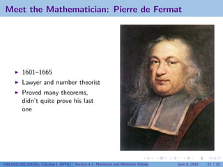
![Extreme values of an algebraic function
Example
Find the extreme values of f (x) = 4 − x 2 on [−2, 1].
Solution
x
We have f (x) = − √ , which is zero when x = 0. (f is not
4 − x2
differentiable at ±2 as well.) So our points to check are:
f (−2) = 0 (absolute min)
f (0) = 2 (absolute max)
√
f (1) = 3
V63.0121.002.2010Su, Calculus I (NYU) Section 4.1 Maximum and Minimum Values June 8, 2010 31 / 32](https://image.slidesharecdn.com/lesson18-maximumandminimumvaluesslides-100610135316-phpapp01-121002231606-phpapp02/85/Lesson18-maximum_and_minimum_values_slides-92-320.jpg)

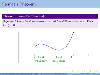
This document is a section from a Calculus I course at New York University covering maximum and minimum values. It begins with announcements about exams and assignments. The objectives are to understand the Extreme Value Theorem and Fermat's Theorem, and use the Closed Interval Method to find extreme values. The document then covers the definitions of extreme points/values and the statements of the Extreme Value Theorem and Fermat's Theorem. It provides examples to illustrate the necessity of the hypotheses in the theorems. The focus is on using calculus concepts like continuity and differentiability to determine maximum and minimum values of functions on closed intervals.