This chapter discusses continuous random variables and their probability density functions. It introduces the normal and exponential distributions and how to calculate probabilities and descriptive statistics for continuous random variables. It also shows how to approximate the binomial distribution using the normal distribution. The chapter objectives are to introduce continuous random variables, discuss the normal distribution and standard normal table, and demonstrate the normal approximation to the binomial distribution.

1. INTRODUCTORY MATHEMATICALINTRODUCTORY MATHEMATICAL
ANALYSISANALYSISFor Business, Economics, and the Life and Social Sciences
©2007 Pearson Education Asia
Chapter 16Chapter 16
Continuous Random VariablesContinuous Random Variables

2. ©2007 Pearson Education Asia
INTRODUCTORY MATHEMATICAL
ANALYSIS
0. Review of Algebra
1. Applications and More Algebra
2. Functions and Graphs
3. Lines, Parabolas, and Systems
4. Exponential and Logarithmic Functions
5. Mathematics of Finance
6. Matrix Algebra
7. Linear Programming
8. Introduction to Probability and Statistics

3. ©2007 Pearson Education Asia
9. Additional Topics in Probability
10. Limits and Continuity
11. Differentiation
12. Additional Differentiation Topics
13. Curve Sketching
14. Integration
15. Methods and Applications of Integration
16. Continuous Random Variables
17. Multivariable Calculus
INTRODUCTORY MATHEMATICAL
ANALYSIS

4. ©2007 Pearson Education Asia
• To introduce continuous random variables and
discuss density functions.
• To discuss the normal distribution, standard
units, and the table of areas under the standard
normal curve.
• To show the technique of estimating the
binomial distribution by using normal
distribution.
Chapter 16: Continuous Random Variables
Chapter ObjectivesChapter Objectives

5. ©2007 Pearson Education Asia
Continuous Random Variables
The Normal Distribution
The Normal Approximation to the Binomial Distributi
16.1)
16.2)
16.3)
Chapter 16: Continuous Random Variables
Chapter OutlineChapter Outline

6. ©2007 Pearson Education Asia
Chapter 16: Continuous Random Variables
16.1 Continuous Random Variables16.1 Continuous Random Variables
• If X is a continuous random variable, the
(probability) density function for X has the
following properties:
( )
( )
( ) ( )∫
∫
=≤≤
=
≥
∞
∞−
b
a
dxxfbXa. P
dxxf.
x. f
3
12
01

7. ©2007 Pearson Education Asia
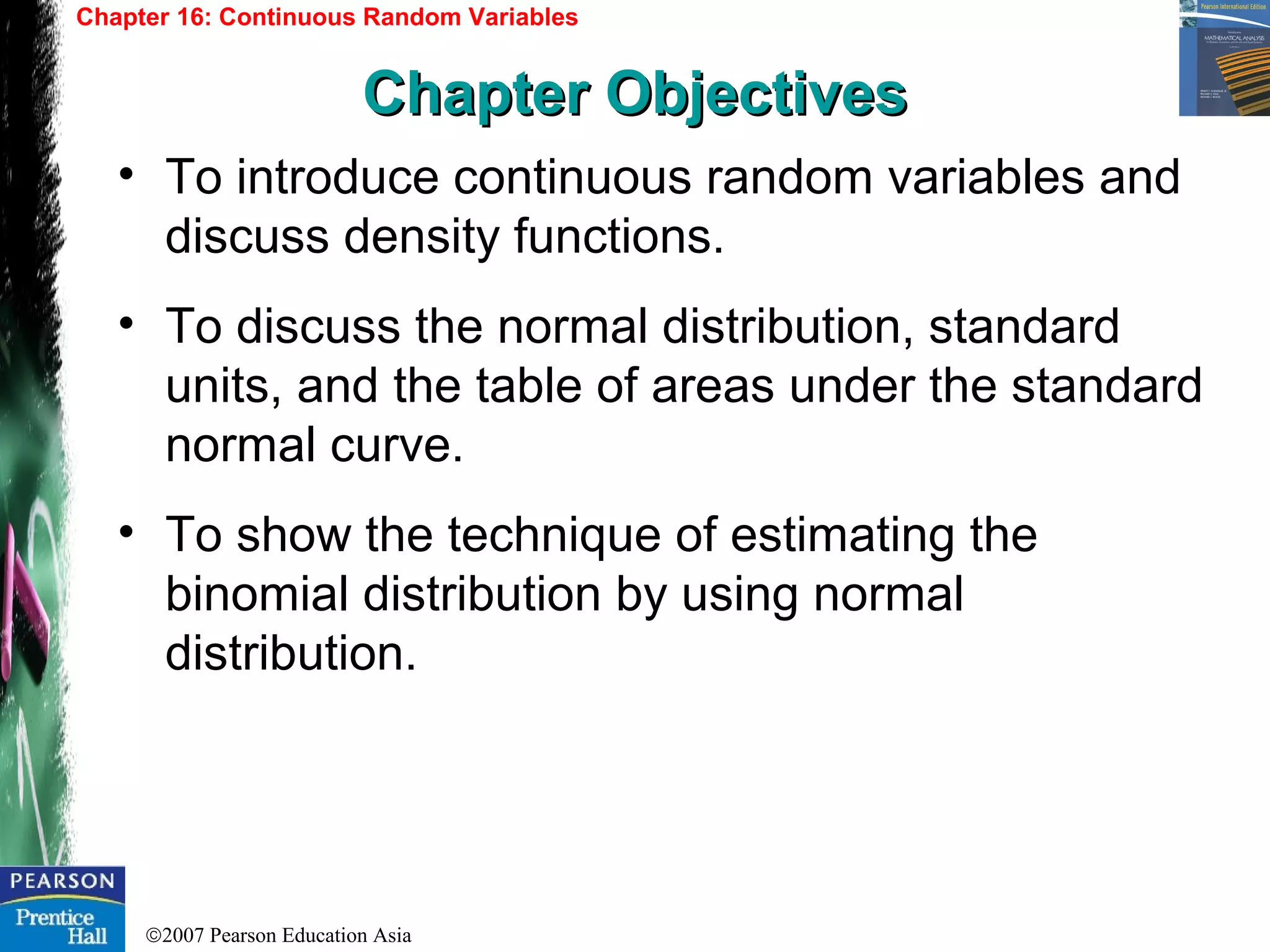
Chapter 16: Continuous Random Variables
16.1 Continuous Random Variables
Example 1 – Uniform Density Function
The uniform density function over [a, b] for the
random variable X is given by
Find P(2 < X < 3).
Solution: If [c, d] is any interval within [a, b] then
For a = 1, b = 4, c = 2, and d = 3,
( )




≤≤
−=
otherwise0
baif
1
x
abxf
( ) ( )
ab
cd
ab
x
dx
ab
dxxfdXcP
d
c
d
c
d
c
−
−
=
−
=
−
==≤≤ ∫∫
1
( )
3
1
14
23
32 =
−
−
=<< XP

8. ©2007 Pearson Education Asia
Chapter 16: Continuous Random Variables
16.1 Continuous Random Variables
Example 3 – Exponential Density Function
The exponential density function is defined by
where k is a positive constant, called a parameter,
whose value depends on the experiment under
consideration. If X is a random variable with this
density function, then X is said to have an
exponential distribution. Let k = 1. Then f(x) = e−x
for x ≥ 0, and f(x) = 0 for x < 0.
( )



<
≥
=
−
0if0
0if
x
xke
xf
kx

9. ©2007 Pearson Education Asia
Chapter 16: Continuous Random Variables
16.1 Continuous Random Variables
Example 3 – Exponential Density Function
a. Find P(2 < X < 3).
Solution:
b. Find P(X > 4).
Solution:
( )
086.0)(
32
3223
3
2
3
2
≈−=−−−=
==<<
−−−−
−−
∫
eeee
edxeXP xx
( )
018.00
1
lim
lim4
44
44
≈+=





+−=
==>
−−
∞→
−
∞
∞→
−
∫∫
ee
e
dxedxeXP
rr
r
x
r
x

10. ©2007 Pearson Education Asia
Chapter 16: Continuous Random Variables
16.1 Continuous Random Variables
Example 5 – Finding the Mean and Standard
Deviation
If X is a random variable with density function given
by
find its mean and standard deviation.
Solution:
( )


 ≤≤
=
otherwise0
20if2
1
xx
xf
( )
3
4
62
1
Mean,
2
0
32
0
=





=





== ∫∫
∞
∞−
x
dxxxdxxxfμ
( )
9
2
9
16
83
4
2
1
2
0
422
0
2222
=−





=





−





=−= ∫∫
∞
∞−
x
dxxxμdxxfxσ
3
2
9
2
Deviation,Standard ==σ

11. ©2007 Pearson Education Asia
Chapter 16: Continuous Random Variables
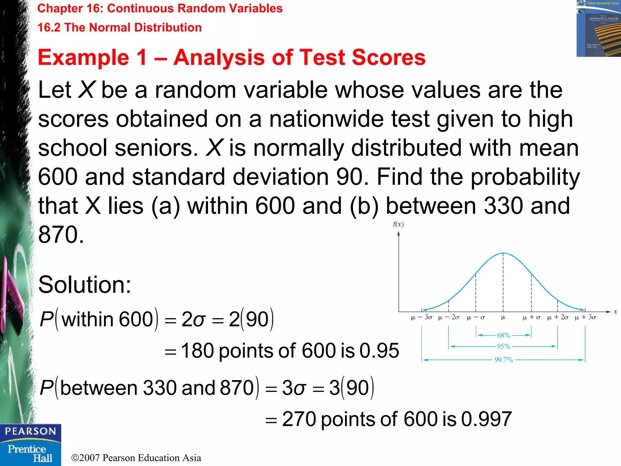
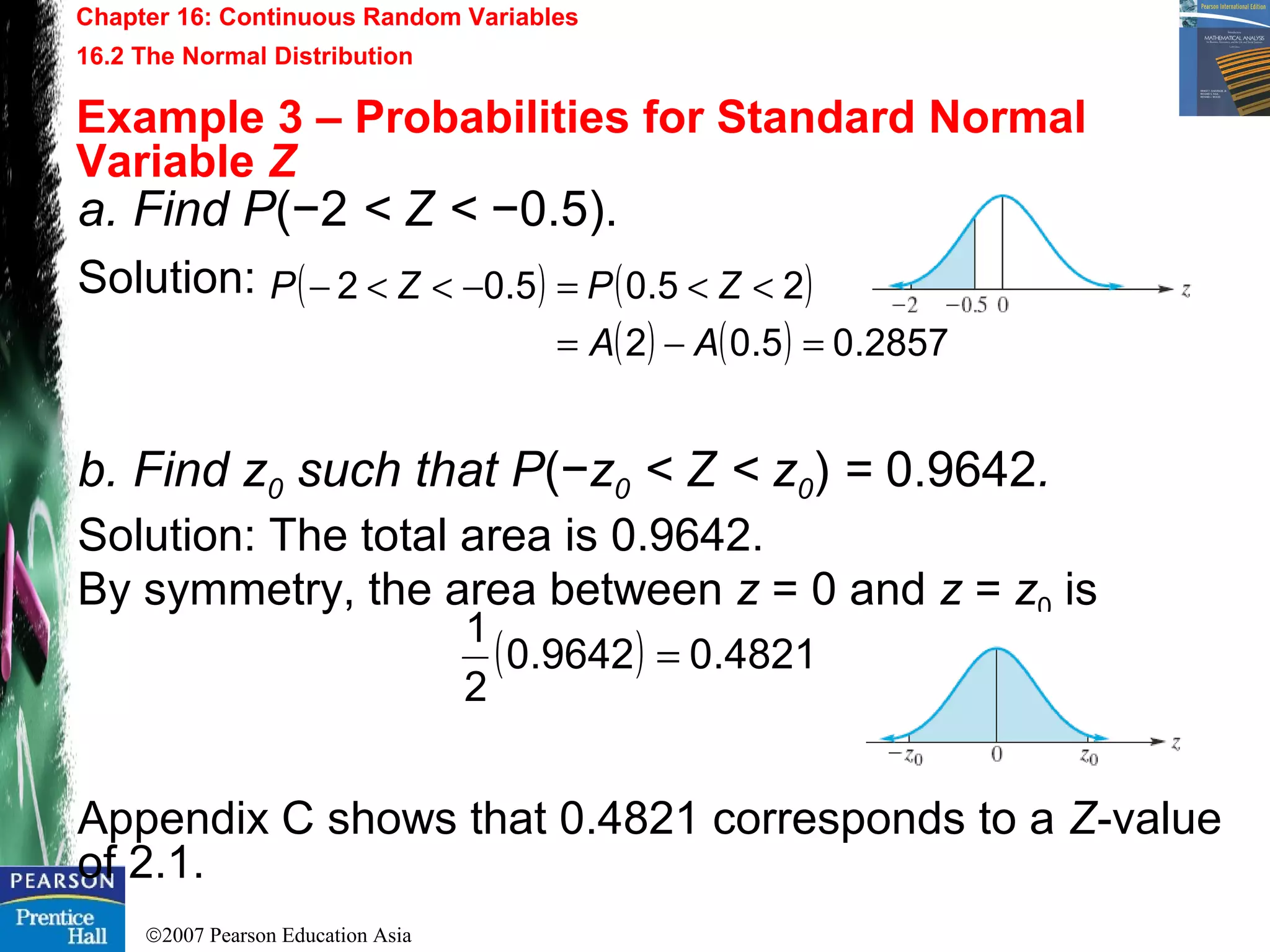
16.2 The Normal Distribution16.2 The Normal Distribution
• Continuous random variable X has a normal distribution if
its density function is given by
called the normal density function.
• Continuous random variable Z has a standard normal
distribution if its density function is given by
called the standard normal density function.
( ) ( ) ( )[ ]
∞<<∞−= −−
xe
πσ
xf σμx
2
1 2
/2/1
( ) 2/2
2
1 z
e
πσ
zf −
=

12. ©2007 Pearson Education Asia
Chapter 16: Continuous Random Variables
16.2 The Normal Distribution
Example 1 – Analysis of Test Scores
Let X be a random variable whose values are the
scores obtained on a nationwide test given to high
school seniors. X is normally distributed with mean
600 and standard deviation 90. Find the probability
that X lies (a) within 600 and (b) between 330 and
870.
Solution:
( ) ( )
0.95is600ofpoints180
9022600within
=
== σP
( ) ( )
0.997is600ofpoints270
9033870and330between
=
== σP

13. ©2007 Pearson Education Asia
Chapter 16: Continuous Random Variables
16.2 The Normal Distribution
Example 3 – Probabilities for Standard Normal
Variable Z
a. Find P(−2 < Z < −0.5).
Solution:
b. Find z0 such that P(−z0 < Z < z0) = 0.9642.
Solution: The total area is 0.9642.
By symmetry, the area between z = 0 and z = z0 is
Appendix C shows that 0.4821 corresponds to a Z-value
of 2.1.
( ) ( )
( ) ( ) 2857.05.02
25.05.02
=−=
<<=−<<−
AA
ZPZP
( ) 4821.09642.0
2
1
=

14. ©2007 Pearson Education Asia
Chapter 16: Continuous Random Variables
16.3 The Normal Approximation to the16.3 The Normal Approximation to the
Binomial DistributionBinomial Distribution
Example 1 – Normal Approximation to a Binomial
Distribution
• The probability of x successes is given by
( ) xnx
xn qpCxXP −
==
Suppose X is a binomial random variable with n =
100 and p = 0.3. Estimate P(X = 40) by using the
normal approximation.
Solution: We have
We use a normal distribution with
( ) ( ) ( )6040
40100 7.03.040 CXP ==
( )
( ) 58.421)7.0(3.0100
303.0100
≈===
===
npqσ
npμ

15. ©2007 Pearson Education Asia
Chapter 16: Continuous Random Variables
16.3 The Normal Approximation to the Binomial Distribution
Example 1 – Normal Approximation to a Binomial Distribution
Solution (cont’d):
Converting 39.5 and 40.5 to Z-values gives
Therefore, ( ) ( )
( ) ( )
0082.0
4808.04890.0
07.229.2
29.207.240
=
−=
−=
≤≤≈=
AA
ZPXP
29.2
21
305.40
and07.2
21
305.39
21 ≈
−
=≈
−
= zz