SlideShare a Scribd company logo
Section 2.8
 Linear Approximation and Differentials

                V63.0121.002.2010Su, Calculus I

                         New York University


                         May 26, 2010


Announcements

   Quiz 2 Thursday on Sections 1.5–2.5
   No class Monday, May 31
   Assignment 2 due Tuesday, June 1

                                               .   .   .   .   .   .
Announcements


           Quiz 2 Thursday on
           Sections 1.5–2.5
           No class Monday, May 31
           Assignment 2 due
           Tuesday, June 1


                                                                           .   .   .     .      .     .

V63.0121.002.2010Su, Calculus I (NYU)   Section 2.8 Linear Approximation               May 26, 2010       2 / 27
Objectives
           Use tangent lines to make
           linear approximations to a
           function.
                   Given a function and a
                   point in the domain,
                   compute the
                   linearization of the
                   function at that point.
                   Use linearization to
                   approximate values of
                   functions
           Given a function, compute
           the differential of that
           function
           Use the differential
           notation to estimate error
           in linear approximations.                                       .   .   .     .      .     .

V63.0121.002.2010Su, Calculus I (NYU)   Section 2.8 Linear Approximation               May 26, 2010       3 / 27
Outline


 The linear approximation of a function near a point
   Examples
   Questions


 Differentials
     Using differentials to estimate error


 Advanced Examples


                                                                           .   .   .     .      .     .

V63.0121.002.2010Su, Calculus I (NYU)   Section 2.8 Linear Approximation               May 26, 2010       4 / 27
The Big Idea

 Question
 Let f be differentiable at a. What linear function best approximates f
 near a?


                                                                           .   .   .     .      .     .

V63.0121.002.2010Su, Calculus I (NYU)   Section 2.8 Linear Approximation               May 26, 2010       5 / 27
The Big Idea

 Question
 Let f be differentiable at a. What linear function best approximates f
 near a?

 Answer
 The tangent line, of course!

 Question
 What is the equation for the line tangent to y = f(x) at (a, f(a))?

 Answer

                                        L(x) = f(a) + f′ (a)(x − a)

                                                                              .   .   .     .      .     .

V63.0121.002.2010Su, Calculus I (NYU)      Section 2.8 Linear Approximation               May 26, 2010       5 / 27
The tangent line is a linear approximation


                                                              y
                                                              .


        L(x) = f(a) + f′ (a)(x − a)

  is a decent approximation to f                      L
                                                      . (x)                              .
  near a.                                              f
                                                       .(x)                              .

                                                       f
                                                       .(a)                .
                                                                               .
                                                                               x−a


                                                               .                                       x
                                                                                                       .
                                                                           a
                                                                           .         x
                                                                                     .

                                                                               .     .       .     .       .    .

V63.0121.002.2010Su, Calculus I (NYU)   Section 2.8 Linear Approximation                         May 26, 2010       6 / 27
The tangent line is a linear approximation


                                                              y
                                                              .


        L(x) = f(a) + f′ (a)(x − a)

  is a decent approximation to f                      L
                                                      . (x)                              .
  near a.                                              f
                                                       .(x)                              .
  How decent? The closer x is to
  a, the better the approxmation                       f
                                                       .(a)                .
                                                                               .
                                                                               x−a
  L(x) is to f(x)

                                                               .                                       x
                                                                                                       .
                                                                           a
                                                                           .         x
                                                                                     .

                                                                               .     .       .     .       .    .

V63.0121.002.2010Su, Calculus I (NYU)   Section 2.8 Linear Approximation                         May 26, 2010       6 / 27
Example
 .
 Example
 Estimate sin(61◦ ) = sin(61π/180) by using a linear approximation
 (i) about a = 0     (ii) about a = 60◦ = π/3.


 .

                                                                           .   .   .     .      .     .

V63.0121.002.2010Su, Calculus I (NYU)   Section 2.8 Linear Approximation               May 26, 2010       7 / 27
Example
 .
 Example
 Estimate sin(61◦ ) = sin(61π/180) by using a linear approximation
 (i) about a = 0     (ii) about a = 60◦ = π/3.


 Solution (i)

        If f(x) = sin x, then f(0) = 0
        and f′ (0) = 1.
        So the linear approximation
        near 0 is L(x) = 0 + 1 · x = x.
        Thus
             (      )
                61π       61π
         sin           ≈       ≈ 1.06465
                180       180

 .

                                                                           .   .   .     .      .     .

V63.0121.002.2010Su, Calculus I (NYU)   Section 2.8 Linear Approximation               May 26, 2010       7 / 27
Example
 .
 Example
 Estimate sin(61◦ ) = sin(61π/180) by using a linear approximation
 (i) about a = 0     (ii) about a = 60◦ = π/3.


 Solution (i)                                              Solution (ii)
                                                                               (π)
                                                                  We have f            =         and
        If f(x) = sin x, then f(0) = 0                              ( )            3
        and f′ (0) = 1.                                           f′ π = .
                                                                     3
        So the linear approximation
        near 0 is L(x) = 0 + 1 · x = x.
        Thus
             (      )
                61π       61π
         sin           ≈       ≈ 1.06465
                180       180

 .

                                                                           .   .       .     .         .   .

V63.0121.002.2010Su, Calculus I (NYU)   Section 2.8 Linear Approximation                   May 26, 2010        7 / 27
Example
 .
 Example
 Estimate sin(61◦ ) = sin(61π/180) by using a linear approximation
 (i) about a = 0     (ii) about a = 60◦ = π/3.


 Solution (i)                                              Solution (ii)
                                                                               (π)         √
                                                                                            3
                                                                  We have f            =            and
        If f(x) = sin x, then f(0) = 0                              ( )            3       2
        and f′ (0) = 1.                                           f′ π = .
                                                                     3
        So the linear approximation
        near 0 is L(x) = 0 + 1 · x = x.
        Thus
             (      )
                61π       61π
         sin           ≈       ≈ 1.06465
                180       180

 .

                                                                           .   .       .        .         .   .

V63.0121.002.2010Su, Calculus I (NYU)   Section 2.8 Linear Approximation                    May 26, 2010          7 / 27
Example
 .
 Example
 Estimate sin(61◦ ) = sin(61π/180) by using a linear approximation
 (i) about a = 0     (ii) about a = 60◦ = π/3.


 Solution (i)                                              Solution (ii)
                                                                               (π)         √
                                                                                            3
                                                                  We have f            =            and
        If f(x) = sin x, then f(0) = 0                              ( )            3       2
        and f′ (0) = 1.                                           f′ π = 1 .
                                                                     3   2
        So the linear approximation
                                                                  So L(x) =
        near 0 is L(x) = 0 + 1 · x = x.
        Thus
             (      )
                61π       61π
         sin           ≈       ≈ 1.06465
                180       180

 .

                                                                           .   .       .        .         .   .

V63.0121.002.2010Su, Calculus I (NYU)   Section 2.8 Linear Approximation                    May 26, 2010          7 / 27
Example
 .
 Example
 Estimate sin(61◦ ) = sin(61π/180) by using a linear approximation
 (i) about a = 0     (ii) about a = 60◦ = π/3.


 Solution (i)                                              Solution (ii)
                                                                               (π)         √
                                                                                            3
                                                                  We have f            =            and
        If f(x) = sin x, then f(0) = 0                              ( )            3       2
        and f′ (0) = 1.                                           f′ π = 1 .
                                                                     3   2         √
        So the linear approximation                                                  3 1(    π)
                                                                  So L(x) =           +   x−
        near 0 is L(x) = 0 + 1 · x = x.                                             2   2    3
        Thus
             (      )
                61π       61π
         sin           ≈       ≈ 1.06465
                180       180

 .

                                                                           .   .       .        .         .   .

V63.0121.002.2010Su, Calculus I (NYU)   Section 2.8 Linear Approximation                    May 26, 2010          7 / 27
Example
 .
 Example
 Estimate sin(61◦ ) = sin(61π/180) by using a linear approximation
 (i) about a = 0     (ii) about a = 60◦ = π/3.


 Solution (i)                                              Solution (ii)
                                                                                     (π)         √
                                                                                                  3
                                                                  We have f                  =             and
        If f(x) = sin x, then f(0) = 0                              ( )                  3       2
        and f′ (0) = 1.                                           f′ π = 1 .
                                                                     3   2               √
        So the linear approximation                                                        3 1(    π)
                                                                  So L(x) =                 +   x−
        near 0 is L(x) = 0 + 1 · x = x.                                                   2   2    3
        Thus                                                      Thus
             (      )                                                            (           )
                61π       61π                                                        61π
         sin           ≈       ≈ 1.06465                                   sin                   ≈
                180       180                                                        180


 .

                                                                            .        .       .         .         .   .

V63.0121.002.2010Su, Calculus I (NYU)   Section 2.8 Linear Approximation                             May 26, 2010        7 / 27
Example
 .
 Example
 Estimate sin(61◦ ) = sin(61π/180) by using a linear approximation
 (i) about a = 0     (ii) about a = 60◦ = π/3.


 Solution (i)                                              Solution (ii)
                                                                                     (π)          √
                                                                                                   3
                                                                  We have f                  =             and
        If f(x) = sin x, then f(0) = 0                              ( )                  3        2
        and f′ (0) = 1.                                           f′ π = 1 .
                                                                     3   2               √
        So the linear approximation                                                        3 1(    π)
                                                                  So L(x) =                 +   x−
        near 0 is L(x) = 0 + 1 · x = x.                                                   2   2    3
        Thus                                                      Thus
             (      )                                                            (           )
                61π       61π                                                        61π
         sin           ≈       ≈ 1.06465                                   sin                   ≈ 0.87475
                180       180                                                        180


 .

                                                                            .        .       .         .         .   .

V63.0121.002.2010Su, Calculus I (NYU)   Section 2.8 Linear Approximation                           May 26, 2010          7 / 27
Example
 .
 Example
 Estimate sin(61◦ ) = sin(61π/180) by using a linear approximation
 (i) about a = 0     (ii) about a = 60◦ = π/3.


 Solution (i)                                              Solution (ii)
                                                                                     (π)          √
                                                                                                   3
                                                                  We have f                  =             and
        If f(x) = sin x, then f(0) = 0                              ( )                  3        2
        and f′ (0) = 1.                                           f′ π = 1 .
                                                                     3   2               √
        So the linear approximation                                                        3 1(    π)
                                                                  So L(x) =                 +   x−
        near 0 is L(x) = 0 + 1 · x = x.                                                   2   2    3
        Thus                                                      Thus
             (      )                                                            (           )
                61π       61π                                                        61π
         sin           ≈       ≈ 1.06465                                   sin                   ≈ 0.87475
                180       180                                                        180


 Calculator check: sin(61◦ ) ≈
 .

                                                                            .        .       .         .         .   .

V63.0121.002.2010Su, Calculus I (NYU)   Section 2.8 Linear Approximation                           May 26, 2010          7 / 27
Example
 .
 Example
 Estimate sin(61◦ ) = sin(61π/180) by using a linear approximation
 (i) about a = 0     (ii) about a = 60◦ = π/3.


 Solution (i)                                              Solution (ii)
                                                                                     (π)          √
                                                                                                   3
                                                                  We have f                  =             and
        If f(x) = sin x, then f(0) = 0                              ( )                  3        2
        and f′ (0) = 1.                                           f′ π = 1 .
                                                                     3   2               √
        So the linear approximation                                                        3 1(    π)
                                                                  So L(x) =                 +   x−
        near 0 is L(x) = 0 + 1 · x = x.                                                   2   2    3
        Thus                                                      Thus
             (      )                                                            (           )
                61π       61π                                                        61π
         sin           ≈       ≈ 1.06465                                   sin                   ≈ 0.87475
                180       180                                                        180


 Calculator check: sin(61◦ ) ≈ 0.87462.
 .

                                                                            .        .       .         .         .   .

V63.0121.002.2010Su, Calculus I (NYU)   Section 2.8 Linear Approximation                           May 26, 2010          7 / 27
Illustration

          y
          .


                                                                     y
                                                                     . = sin x


          .                                                                        x
                                                                                   .
                                                 . 1◦
                                                 6
                                                                           .   .       .     .      .     .

V63.0121.002.2010Su, Calculus I (NYU)   Section 2.8 Linear Approximation                   May 26, 2010       8 / 27
Illustration

          y
          .
                                                                  y
                                                                  . = L1 (x) = x


                                                                     y
                                                                     . = sin x


          .                                                                        x
                                                                                   .
              0
              .                                  . 1◦
                                                 6
                                                                           .   .       .     .      .     .

V63.0121.002.2010Su, Calculus I (NYU)   Section 2.8 Linear Approximation                   May 26, 2010       8 / 27
Illustration

          y
          .
                                                                  y
                                                                  . = L1 (x) = x


                           b
                           . ig difference!                          y
                                                                     . = sin x


          .                                                                        x
                                                                                   .
              0
              .                                  . 1◦
                                                 6
                                                                           .   .       .     .      .     .

V63.0121.002.2010Su, Calculus I (NYU)   Section 2.8 Linear Approximation                   May 26, 2010       8 / 27
Illustration

          y
          .
                                                                  y
                                                                  . = L1 (x) = x


                                                                                   √                   (            )
                                                                  y
                                                                  . = L2 (x) =     2
                                                                                    3
                                                                                           +       1
                                                                                                   2       x−   π
                                                                                                                3
                                                                    y
                                                                    . = sin x
                                               .


          .                                    .                                   x
                                                                                   .
              0
              .                         .
                                        π/3        . 1◦
                                                   6
                                                                           .   .       .       .           .        .

V63.0121.002.2010Su, Calculus I (NYU)   Section 2.8 Linear Approximation                   May 26, 2010                 8 / 27
Illustration

          y
          .
                                                                  y
                                                                  . = L1 (x) = x


                                                                                   √                   (            )
                                                               y
                                                               . = L2 (x) =        2
                                                                                    3
                                                                                           +       1
                                                                                                   2       x−   π
                                                                                                                3
                                                                 y
                                                                 . = sin x
                                               . . ery little difference!
                                                 v


          .                                    .                                   x
                                                                                   .
              0
              .                         .
                                        π/3        . 1◦
                                                   6
                                                                           .   .       .       .           .        .

V63.0121.002.2010Su, Calculus I (NYU)   Section 2.8 Linear Approximation                   May 26, 2010                 8 / 27
Another Example

 Example
                 √
 Estimate         10 using the fact that 10 = 9 + 1.


                                                                           .   .   .     .      .     .

V63.0121.002.2010Su, Calculus I (NYU)   Section 2.8 Linear Approximation               May 26, 2010       9 / 27
Another Example

 Example
                 √
 Estimate         10 using the fact that 10 = 9 + 1.

 Solution
                                                                                   √
 The key step is to use a linear approximation to f(x) =
                     √                                                              x near a = 9
 to estimate f(10) = 10.


                                                                           .   .   .     .      .     .

V63.0121.002.2010Su, Calculus I (NYU)   Section 2.8 Linear Approximation               May 26, 2010       9 / 27
Another Example

 Example
                 √
 Estimate         10 using the fact that 10 = 9 + 1.

 Solution
                                                                                   √
 The key step is to use a linear approximation to f(x) =
                     √                                                              x near a = 9
 to estimate f(10) = 10.
                               √    √     d√
                                10 ≈ 9 +      x     (1)
                                          dx    x=9
                                         1        19
                                   =3+      (1) =     ≈ 3.167
                                       2·3         6


                                                                           .   .   .     .      .     .

V63.0121.002.2010Su, Calculus I (NYU)   Section 2.8 Linear Approximation               May 26, 2010       9 / 27
Another Example

 Example
                 √
 Estimate         10 using the fact that 10 = 9 + 1.

 Solution
                                                                                   √
 The key step is to use a linear approximation to f(x) =
                     √                                                              x near a = 9
 to estimate f(10) = 10.
                                √    √     d√
                                 10 ≈ 9 +      x     (1)
                                           dx    x=9
                                          1        19
                                    =3+      (1) =     ≈ 3.167
                                        2·3         6

              (        )2
                  19
 Check:                     =
                  6
                                                                           .   .   .     .      .     .

V63.0121.002.2010Su, Calculus I (NYU)   Section 2.8 Linear Approximation               May 26, 2010       9 / 27
Another Example

 Example
                 √
 Estimate         10 using the fact that 10 = 9 + 1.

 Solution
                                                                                   √
 The key step is to use a linear approximation to f(x) =
                     √                                                              x near a = 9
 to estimate f(10) = 10.
                                √    √     d√
                                 10 ≈ 9 +      x     (1)
                                           dx    x=9
                                          1        19
                                    =3+      (1) =     ≈ 3.167
                                        2·3         6

              (        )2
                  19            361
 Check:                     =       .
                  6             36
                                                                           .   .   .     .      .     .

V63.0121.002.2010Su, Calculus I (NYU)   Section 2.8 Linear Approximation               May 26, 2010       9 / 27
Dividing without dividing?
 Example
 Suppose I have an irrational fear of division and need to estimate
 577 ÷ 408. I write
                         577            1             1  1
                             = 1 + 169     = 1 + 169 × ×    .
                         408           408            4 102
                                         1
 But still I have to find                   .
                                        102


                                                                               .   .   .      .      .    .

V63.0121.002.2010Su, Calculus I (NYU)       Section 2.8 Linear Approximation               May 26, 2010   10 / 27
Dividing without dividing?
 Example
 Suppose I have an irrational fear of division and need to estimate
 577 ÷ 408. I write
                         577            1             1  1
                             = 1 + 169     = 1 + 169 × ×    .
                         408           408            4 102
                                         1
 But still I have to find                   .
                                        102

 Solution
                  1
 Let f(x) =         . We know f(100) and we want to estimate f(102).
                  x
                                                                  1   1
             f(102) ≈ f(100) + f′ (100)(2) =                        −     (2) = 0.0098
                                                                 100 1002
                                                    577
                                            =⇒          ≈ 1.41405
                                                    408                        .   .   .      .      .    .

V63.0121.002.2010Su, Calculus I (NYU)       Section 2.8 Linear Approximation               May 26, 2010   10 / 27
Questions

 Example
 Suppose we are traveling in a car and at noon our speed is 50 mi/hr.
 How far will we have traveled by 2:00pm? by 3:00pm? By midnight?


                                                                           .   .   .     .      .     .

V63.0121.002.2010Su, Calculus I (NYU)   Section 2.8 Linear Approximation               May 26, 2010   11 / 27
Answers


 Example
 Suppose we are traveling in a car and at noon our speed is 50 mi/hr.
 How far will we have traveled by 2:00pm? by 3:00pm? By midnight?


                                                                           .   .   .      .      .    .

V63.0121.002.2010Su, Calculus I (NYU)   Section 2.8 Linear Approximation               May 26, 2010   12 / 27
Answers


 Example
 Suppose we are traveling in a car and at noon our speed is 50 mi/hr.
 How far will we have traveled by 2:00pm? by 3:00pm? By midnight?

 Answer

         100 mi
         150 mi
         600 mi (?) (Is it reasonable to assume 12 hours at the same
         speed?)


                                                                           .   .   .      .      .    .

V63.0121.002.2010Su, Calculus I (NYU)   Section 2.8 Linear Approximation               May 26, 2010   12 / 27
Questions

 Example
 Suppose we are traveling in a car and at noon our speed is 50 mi/hr.
 How far will we have traveled by 2:00pm? by 3:00pm? By midnight?

 Example
 Suppose our factory makes MP3 players and the marginal cost is
 currently $50/lot. How much will it cost to make 2 more lots? 3 more
 lots? 12 more lots?


                                                                           .   .   .      .      .    .

V63.0121.002.2010Su, Calculus I (NYU)   Section 2.8 Linear Approximation               May 26, 2010   13 / 27
Answers


 Example
 Suppose our factory makes MP3 players and the marginal cost is
 currently $50/lot. How much will it cost to make 2 more lots? 3 more
 lots? 12 more lots?

 Answer

         $100
         $150
         $600 (?)


                                                                           .   .   .      .      .    .

V63.0121.002.2010Su, Calculus I (NYU)   Section 2.8 Linear Approximation               May 26, 2010   14 / 27
Questions

 Example
 Suppose we are traveling in a car and at noon our speed is 50 mi/hr.
 How far will we have traveled by 2:00pm? by 3:00pm? By midnight?

 Example
 Suppose our factory makes MP3 players and the marginal cost is
 currently $50/lot. How much will it cost to make 2 more lots? 3 more
 lots? 12 more lots?

 Example
 Suppose a line goes through the point (x0 , y0 ) and has slope m. If the
 point is moved horizontally by dx, while staying on the line, what is the
 corresponding vertical movement?

                                                                           .   .   .      .      .    .

V63.0121.002.2010Su, Calculus I (NYU)   Section 2.8 Linear Approximation               May 26, 2010   15 / 27
Answers


 Example
 Suppose a line goes through the point (x0 , y0 ) and has slope m. If the
 point is moved horizontally by dx, while staying on the line, what is the
 corresponding vertical movement?


                                                                           .   .   .      .      .    .

V63.0121.002.2010Su, Calculus I (NYU)   Section 2.8 Linear Approximation               May 26, 2010   16 / 27
Answers


 Example
 Suppose a line goes through the point (x0 , y0 ) and has slope m. If the
 point is moved horizontally by dx, while staying on the line, what is the
 corresponding vertical movement?

 Answer
 The slope of the line is
                                      rise
                                                m=
                                      run
 We are given a “run” of dx, so the corresponding “rise” is m dx.


                                                                           .   .   .      .      .    .

V63.0121.002.2010Su, Calculus I (NYU)   Section 2.8 Linear Approximation               May 26, 2010   16 / 27
Outline


 The linear approximation of a function near a point
   Examples
   Questions


 Differentials
     Using differentials to estimate error


 Advanced Examples


                                                                           .   .   .      .      .    .

V63.0121.002.2010Su, Calculus I (NYU)   Section 2.8 Linear Approximation               May 26, 2010   17 / 27
Differentials are another way to express derivatives


       f(x + ∆x) − f(x) ≈ f′ (x) ∆x                            y
                                                               .
                  ∆y                    dy

  Rename ∆x = dx, so we can
  write this as
                                                                                       .
             ∆y ≈ dy = f′ (x)dx.                                                                .
                                                                                                dy
                                                                                           .
                                                                                           ∆y

  And this looks a lot like the                                             .
                                                                             .
                                                                             dx = ∆x
  Leibniz-Newton identity

                    dy                                          .
                       = f′ (x)                                                                             x
                                                                                                            .
                    dx                                                      x x
                                                                            . . + ∆x


                                                                             .     .            .       .       .   .

V63.0121.002.2010Su, Calculus I (NYU)    Section 2.8 Linear Approximation                            May 26, 2010   18 / 27
Differentials are another way to express derivatives


       f(x + ∆x) − f(x) ≈ f′ (x) ∆x                            y
                                                               .
                  ∆y                    dy

  Rename ∆x = dx, so we can
  write this as
                                                                                       .
             ∆y ≈ dy = f′ (x)dx.                                                                .
                                                                                                dy
                                                                                           .
                                                                                           ∆y

  And this looks a lot like the                                             .
                                                                             .
                                                                             dx = ∆x
  Leibniz-Newton identity

                    dy                                          .
                       = f′ (x)                                                                             x
                                                                                                            .
                    dx                                                      x x
                                                                            . . + ∆x
 Linear approximation means ∆y ≈ dy = f′ (x0 ) dx near x0 .
                                                                             .     .            .       .       .   .

V63.0121.002.2010Su, Calculus I (NYU)    Section 2.8 Linear Approximation                            May 26, 2010   18 / 27
Using differentials to estimate error


                                                              y
                                                              .
  If y = f(x), x0 and ∆x is known,
  and an estimate of ∆y is
  desired:
          Approximate: ∆y ≈ dy                                                        .
          Differentiate: dy = f′ (x) dx                                                   .
                                                                                          ∆y
                                                                                               .
                                                                                               dy


          Evaluate at x = x0 and                                           .
                                                                            .
                                                                            dx = ∆x
          dx = ∆x.

                                                               .                                           x
                                                                                                           .
                                                                           x x
                                                                           . . + ∆x

                                                                            .     .            .       .       .   .

V63.0121.002.2010Su, Calculus I (NYU)   Section 2.8 Linear Approximation                            May 26, 2010   19 / 27
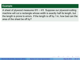
Example
 A sheet of plywood measures 8 ft × 4 ft. Suppose our plywood-cutting
 machine will cut a rectangle whose width is exactly half its length, but
 the length is prone to errors. If the length is off by 1 in, how bad can the
 area of the sheet be off by?


                                                                           .   .   .      .      .    .

V63.0121.002.2010Su, Calculus I (NYU)   Section 2.8 Linear Approximation               May 26, 2010   20 / 27
Example
 A sheet of plywood measures 8 ft × 4 ft. Suppose our plywood-cutting
 machine will cut a rectangle whose width is exactly half its length, but
 the length is prone to errors. If the length is off by 1 in, how bad can the
 area of the sheet be off by?

 Solution
                       1 2
 Write A(ℓ) =            ℓ . We want to know ∆A when ℓ = 8 ft and ∆ℓ = 1 in.
                       2


                                                                           .   .   .      .      .    .

V63.0121.002.2010Su, Calculus I (NYU)   Section 2.8 Linear Approximation               May 26, 2010   20 / 27
Example
 A sheet of plywood measures 8 ft × 4 ft. Suppose our plywood-cutting
 machine will cut a rectangle whose width is exactly half its length, but
 the length is prone to errors. If the length is off by 1 in, how bad can the
 area of the sheet be off by?

 Solution
                1 2
 Write A(ℓ) =     ℓ . We want to know ∆A when ℓ = 8 ft and ∆ℓ = 1 in.
                2      ( )
                         97     9409         9409
     (I) A(ℓ + ∆ℓ) = A       =       So ∆A =       − 32 ≈ 0.6701.
                         12      288          288


                                                                           .   .   .      .      .    .

V63.0121.002.2010Su, Calculus I (NYU)   Section 2.8 Linear Approximation               May 26, 2010   20 / 27
Example
 A sheet of plywood measures 8 ft × 4 ft. Suppose our plywood-cutting
 machine will cut a rectangle whose width is exactly half its length, but
 the length is prone to errors. If the length is off by 1 in, how bad can the
 area of the sheet be off by?

 Solution
                 1 2
 Write A(ℓ) =      ℓ . We want to know ∆A when ℓ = 8 ft and ∆ℓ = 1 in.
                 2      ( )
                          97      9409            9409
     (I) A(ℓ + ∆ℓ) = A         =       So ∆A =         − 32 ≈ 0.6701.
                          12      288             288
         dA
    (II)     = ℓ, so dA = ℓ dℓ, which should be a good estimate for ∆ℓ.
         dℓ
         When ℓ = 8 and dℓ = 12 , we have dA = 12 = 2 ≈ 0.667. So we
                                1                  8
                                                       3
         get estimates close to the hundredth of a square foot.

                                                                           .   .   .      .      .    .

V63.0121.002.2010Su, Calculus I (NYU)   Section 2.8 Linear Approximation               May 26, 2010   20 / 27
Why?


 Why use linear approximations dy when the actual difference ∆y is
 known?
         Linear approximation is quick and reliable. Finding ∆y exactly
         depends on the function.
         These examples are overly simple. See the “Advanced Examples”
         later.
         In real life, sometimes only f(a) and f′ (a) are known, and not the
         general f(x).


                                                                           .   .   .      .      .    .

V63.0121.002.2010Su, Calculus I (NYU)   Section 2.8 Linear Approximation               May 26, 2010   21 / 27
Outline


 The linear approximation of a function near a point
   Examples
   Questions


 Differentials
     Using differentials to estimate error


 Advanced Examples


                                                                           .   .   .      .      .    .

V63.0121.002.2010Su, Calculus I (NYU)   Section 2.8 Linear Approximation               May 26, 2010   22 / 27
Gravitation
Pencils down!

 Example

         Drop a 1 kg ball off the roof of the Silver Center (50m high). We
         usually say that a falling object feels a force F = −mg from gravity.


                                                                           .   .   .      .      .    .

V63.0121.002.2010Su, Calculus I (NYU)   Section 2.8 Linear Approximation               May 26, 2010   23 / 27
Gravitation
Pencils down!

 Example

         Drop a 1 kg ball off the roof of the Silver Center (50m high). We
         usually say that a falling object feels a force F = −mg from gravity.
         In fact, the force felt is
                                                              GMm
                                              F(r) = −            ,
                                                               r2
         where M is the mass of the earth and r is the distance from the
         center of the earth to the object. G is a constant.
                                                GMm
         At r = re the force really is F(re ) =      = −mg.
                                                 r2
                                                  e
         What is the maximum error in replacing the actual force felt at the
         top of the building F(re + ∆r) by the force felt at ground level
         F(re )? The relative error? The percentage error?                 .   .   .      .      .    .

V63.0121.002.2010Su, Calculus I (NYU)   Section 2.8 Linear Approximation               May 26, 2010   23 / 27
Gravitation Solution
 Solution
 We wonder if ∆F = F(re + ∆r) − F(re ) is small.
         Using a linear approximation,

                                                dF           GMm
                                  ∆F ≈ dF =           dr = 2 3 dr
                                                dr re         re
                                                (      )
                                                  GMm dr           ∆r
                                              =     2
                                                             = 2mg
                                                   re     re       re

                             ∆F        ∆r
         The relative error is   ≈ −2
                              F        re
         re = 6378.1 km. If ∆r = 50 m,
              ∆F      ∆r         50
                 ≈ −2    = −2         = −1.56 × 10−5 = −0.00156%
               F      re      6378100
                                                                           .   .   .      .      .    .

V63.0121.002.2010Su, Calculus I (NYU)   Section 2.8 Linear Approximation               May 26, 2010   24 / 27
Systematic linear approximation

         √                    √
          2 is irrational, but 9/4 is rational and 9/4 is close to 2.


                                                                           .   .   .      .      .    .

V63.0121.002.2010Su, Calculus I (NYU)   Section 2.8 Linear Approximation               May 26, 2010   25 / 27
Systematic linear approximation

         √                    √
          2 is irrational, but 9/4 is rational and 9/4 is close to 2. So
                          √   √           √                            1                  17
                           2 = 9/4 − 1/4 ≈ 9/4 +                               (−1/4) =
                                                                   2(3/2)                 12


                                                                           .     .   .       .      .    .

V63.0121.002.2010Su, Calculus I (NYU)   Section 2.8 Linear Approximation                  May 26, 2010   25 / 27
Systematic linear approximation

         √                    √
          2 is irrational, but 9/4 is rational and 9/4 is close to 2. So
                          √   √           √                            1                  17
                           2 = 9/4 − 1/4 ≈ 9/4 +                               (−1/4) =
                                                                   2(3/2)                 12


         This is a better approximation since (17/12)2 = 289/144
         Do it again!
             √   √                 √                                    1
              2 = 289/144 − 1/144 ≈ 289/144 +                                 (−1/144) = 577/408
                                                                     2(17/12)
                 (         )2
                     577            332, 929             1
         Now                    =            which is          away from 2.
                     408            166, 464          166, 464

                                                                           .     .   .       .      .    .

V63.0121.002.2010Su, Calculus I (NYU)   Section 2.8 Linear Approximation                  May 26, 2010   25 / 27
Illustration of the previous example


                                   .


                                                                           .   .   .      .      .    .

V63.0121.002.2010Su, Calculus I (NYU)   Section 2.8 Linear Approximation               May 26, 2010   26 / 27
Illustration of the previous example


                                   .


                                                                           .   .   .      .      .    .

V63.0121.002.2010Su, Calculus I (NYU)   Section 2.8 Linear Approximation               May 26, 2010   26 / 27
Illustration of the previous example


                                   .
                                                          2
                                                          .


                                                                           .   .   .      .      .    .

V63.0121.002.2010Su, Calculus I (NYU)   Section 2.8 Linear Approximation               May 26, 2010   26 / 27
Illustration of the previous example


                                                               .


                                   .
                                                          2
                                                          .


                                                                           .   .   .      .      .    .

V63.0121.002.2010Su, Calculus I (NYU)   Section 2.8 Linear Approximation               May 26, 2010   26 / 27
Illustration of the previous example


                                               . 2, 17 )
                                               ( 12
                                                           . .


                                   .
                                                           2
                                                           .


                                                                           .   .   .      .      .    .

V63.0121.002.2010Su, Calculus I (NYU)   Section 2.8 Linear Approximation               May 26, 2010   26 / 27
Illustration of the previous example


                                                                       .
                                        . 2, 17/12)
                                        (
                                                        .                  . 4, 3)
                                                                           (9 2


                                                                            .        .   .      .      .    .

V63.0121.002.2010Su, Calculus I (NYU)   Section 2.8 Linear Approximation                     May 26, 2010   26 / 27
Illustration of the previous example


                                                                       .
                                        . 2, 17/12)
                                        (
                                                        .. (              . 9, 3)
                                                                          (
                                                                          )4 2
                                                               289 17
                                                          .    144 , 12


                                                                            .       .   .      .      .    .

V63.0121.002.2010Su, Calculus I (NYU)   Section 2.8 Linear Approximation                    May 26, 2010   26 / 27
Illustration of the previous example


                                                                 .
                                        . 2, 17/12)
                                        (
                                                    .. (           . 9, 3)
                                                                   (
                                         ( 577 )                  )4 2
                                         . 2, 408        289 17
                                                       . 144 , 12


                                                                           .   .   .      .      .    .

V63.0121.002.2010Su, Calculus I (NYU)   Section 2.8 Linear Approximation               May 26, 2010   26 / 27
Summary


         Linear approximation: If f is differentiable at a, the best linear
         approximation to f near a is given by

                                        Lf,a (x) = f(a) + f′ (a)(x − a)

         Differentials: If f is differentiable at x, a good approximation to
         ∆y = f(x + ∆x) − f(x) is

                                                         dy        dy
                                        ∆y ≈ dy =           · dx =    · ∆x
                                                         dx        dx
         Don’t buy plywood from me.


                                                                             .   .   .      .      .    .

V63.0121.002.2010Su, Calculus I (NYU)     Section 2.8 Linear Approximation               May 26, 2010   27 / 27

More Related Content

What's hot

Nonlinear Manifolds in Computer Vision
Nonlinear Manifolds in Computer VisionNonlinear Manifolds in Computer Vision
Nonlinear Manifolds in Computer Visionzukun
 
11.solution of linear and nonlinear partial differential equations using mixt...
11.solution of linear and nonlinear partial differential equations using mixt...11.solution of linear and nonlinear partial differential equations using mixt...
11.solution of linear and nonlinear partial differential equations using mixt...Alexander Decker
 
Solution of linear and nonlinear partial differential equations using mixture...
Solution of linear and nonlinear partial differential equations using mixture...Solution of linear and nonlinear partial differential equations using mixture...
Solution of linear and nonlinear partial differential equations using mixture...
Alexander Decker
 
11.final paper -0047www.iiste.org call-for_paper-58
11.final paper -0047www.iiste.org call-for_paper-5811.final paper -0047www.iiste.org call-for_paper-58
11.final paper -0047www.iiste.org call-for_paper-58
Alexander Decker
 
Lesson 2: A Catalog of Essential Functions
Lesson 2: A Catalog of Essential FunctionsLesson 2: A Catalog of Essential Functions
Lesson 2: A Catalog of Essential Functions
Matthew Leingang
 
Homotopy perturbation and elzaki transform for solving nonlinear partial diff...
Homotopy perturbation and elzaki transform for solving nonlinear partial diff...Homotopy perturbation and elzaki transform for solving nonlinear partial diff...
Homotopy perturbation and elzaki transform for solving nonlinear partial diff...Alexander Decker
 
11.homotopy perturbation and elzaki transform for solving nonlinear partial d...
11.homotopy perturbation and elzaki transform for solving nonlinear partial d...11.homotopy perturbation and elzaki transform for solving nonlinear partial d...
11.homotopy perturbation and elzaki transform for solving nonlinear partial d...
Alexander Decker
 
Nature-Inspired Metaheuristic Algorithms for Optimization and Computational I...
Nature-Inspired Metaheuristic Algorithms for Optimization and Computational I...Nature-Inspired Metaheuristic Algorithms for Optimization and Computational I...
Nature-Inspired Metaheuristic Algorithms for Optimization and Computational I...
Xin-She Yang
 
Lesson 14: Derivatives of Exponential and Logarithmic Functions (Section 021 ...
Lesson 14: Derivatives of Exponential and Logarithmic Functions (Section 021 ...Lesson 14: Derivatives of Exponential and Logarithmic Functions (Section 021 ...
Lesson 14: Derivatives of Exponential and Logarithmic Functions (Section 021 ...
Matthew Leingang
 
Camera calibration
Camera calibrationCamera calibration
Camera calibration
Yuji Oyamada
 
On the solvability of a system of forward-backward linear equations with unbo...
On the solvability of a system of forward-backward linear equations with unbo...On the solvability of a system of forward-backward linear equations with unbo...
On the solvability of a system of forward-backward linear equations with unbo...
Nikita V. Artamonov
 
Lesson 14: Derivatives of Exponential and Logarithmic Functions (Section 041 ...
Lesson 14: Derivatives of Exponential and Logarithmic Functions (Section 041 ...Lesson 14: Derivatives of Exponential and Logarithmic Functions (Section 041 ...
Lesson 14: Derivatives of Exponential and Logarithmic Functions (Section 041 ...
Matthew Leingang
 
Differential Geometry
Differential GeometryDifferential Geometry
Differential Geometrylapuyade
 
Lesson 13: Exponential and Logarithmic Functions (Section 041 slides)
Lesson 13: Exponential and Logarithmic Functions (Section 041 slides)Lesson 13: Exponential and Logarithmic Functions (Section 041 slides)
Lesson 13: Exponential and Logarithmic Functions (Section 041 slides)
Matthew Leingang
 
Bayesian Core: Chapter 7
Bayesian Core: Chapter 7Bayesian Core: Chapter 7
Bayesian Core: Chapter 7
Christian Robert
 
05 history of cv a machine learning (theory) perspective on computer vision
05  history of cv a machine learning (theory) perspective on computer vision05  history of cv a machine learning (theory) perspective on computer vision
05 history of cv a machine learning (theory) perspective on computer visionzukun
 

What's hot (16)

Nonlinear Manifolds in Computer Vision
Nonlinear Manifolds in Computer VisionNonlinear Manifolds in Computer Vision
Nonlinear Manifolds in Computer Vision
 
11.solution of linear and nonlinear partial differential equations using mixt...
11.solution of linear and nonlinear partial differential equations using mixt...11.solution of linear and nonlinear partial differential equations using mixt...
11.solution of linear and nonlinear partial differential equations using mixt...
 
Solution of linear and nonlinear partial differential equations using mixture...
Solution of linear and nonlinear partial differential equations using mixture...Solution of linear and nonlinear partial differential equations using mixture...
Solution of linear and nonlinear partial differential equations using mixture...
 
11.final paper -0047www.iiste.org call-for_paper-58
11.final paper -0047www.iiste.org call-for_paper-5811.final paper -0047www.iiste.org call-for_paper-58
11.final paper -0047www.iiste.org call-for_paper-58
 
Lesson 2: A Catalog of Essential Functions
Lesson 2: A Catalog of Essential FunctionsLesson 2: A Catalog of Essential Functions
Lesson 2: A Catalog of Essential Functions
 
Homotopy perturbation and elzaki transform for solving nonlinear partial diff...
Homotopy perturbation and elzaki transform for solving nonlinear partial diff...Homotopy perturbation and elzaki transform for solving nonlinear partial diff...
Homotopy perturbation and elzaki transform for solving nonlinear partial diff...
 
11.homotopy perturbation and elzaki transform for solving nonlinear partial d...
11.homotopy perturbation and elzaki transform for solving nonlinear partial d...11.homotopy perturbation and elzaki transform for solving nonlinear partial d...
11.homotopy perturbation and elzaki transform for solving nonlinear partial d...
 
Nature-Inspired Metaheuristic Algorithms for Optimization and Computational I...
Nature-Inspired Metaheuristic Algorithms for Optimization and Computational I...Nature-Inspired Metaheuristic Algorithms for Optimization and Computational I...
Nature-Inspired Metaheuristic Algorithms for Optimization and Computational I...
 
Lesson 14: Derivatives of Exponential and Logarithmic Functions (Section 021 ...
Lesson 14: Derivatives of Exponential and Logarithmic Functions (Section 021 ...Lesson 14: Derivatives of Exponential and Logarithmic Functions (Section 021 ...
Lesson 14: Derivatives of Exponential and Logarithmic Functions (Section 021 ...
 
Camera calibration
Camera calibrationCamera calibration
Camera calibration
 
On the solvability of a system of forward-backward linear equations with unbo...
On the solvability of a system of forward-backward linear equations with unbo...On the solvability of a system of forward-backward linear equations with unbo...
On the solvability of a system of forward-backward linear equations with unbo...
 
Lesson 14: Derivatives of Exponential and Logarithmic Functions (Section 041 ...
Lesson 14: Derivatives of Exponential and Logarithmic Functions (Section 041 ...Lesson 14: Derivatives of Exponential and Logarithmic Functions (Section 041 ...
Lesson 14: Derivatives of Exponential and Logarithmic Functions (Section 041 ...
 
Differential Geometry
Differential GeometryDifferential Geometry
Differential Geometry
 
Lesson 13: Exponential and Logarithmic Functions (Section 041 slides)
Lesson 13: Exponential and Logarithmic Functions (Section 041 slides)Lesson 13: Exponential and Logarithmic Functions (Section 041 slides)
Lesson 13: Exponential and Logarithmic Functions (Section 041 slides)
 
Bayesian Core: Chapter 7
Bayesian Core: Chapter 7Bayesian Core: Chapter 7
Bayesian Core: Chapter 7
 
05 history of cv a machine learning (theory) perspective on computer vision
05  history of cv a machine learning (theory) perspective on computer vision05  history of cv a machine learning (theory) perspective on computer vision
05 history of cv a machine learning (theory) perspective on computer vision
 

Viewers also liked

5-1 Mental Math: Patterns in Multiplication
5-1 Mental Math: Patterns in Multiplication5-1 Mental Math: Patterns in Multiplication
5-1 Mental Math: Patterns in MultiplicationMel Anthony Pepito
 
Lesson 11: Implicit Differentiation
Lesson 11: Implicit DifferentiationLesson 11: Implicit Differentiation
Lesson 11: Implicit Differentiation
Mel Anthony Pepito
 
Lesson 16: Inverse Trigonometric Functions
Lesson 16: Inverse Trigonometric FunctionsLesson 16: Inverse Trigonometric Functions
Lesson 16: Inverse Trigonometric FunctionsMel Anthony Pepito
 
6-2 Multiplying Decimals by Whole Numbers
6-2 Multiplying Decimals by Whole Numbers6-2 Multiplying Decimals by Whole Numbers
6-2 Multiplying Decimals by Whole NumbersMel Anthony Pepito
 
6-1 Mental Math: Multiplying Decimals by 10, 100, 1000
6-1 Mental Math: Multiplying Decimals by 10, 100, 10006-1 Mental Math: Multiplying Decimals by 10, 100, 1000
6-1 Mental Math: Multiplying Decimals by 10, 100, 1000Mel Anthony Pepito
 
Multiply And Divide Decimals By Powers Of 10
Multiply And Divide Decimals By Powers Of 10Multiply And Divide Decimals By Powers Of 10
Multiply And Divide Decimals By Powers Of 10
Brooke Young
 

Viewers also liked (7)

5-1 Mental Math: Patterns in Multiplication
5-1 Mental Math: Patterns in Multiplication5-1 Mental Math: Patterns in Multiplication
5-1 Mental Math: Patterns in Multiplication
 
Lesson 11: Implicit Differentiation
Lesson 11: Implicit DifferentiationLesson 11: Implicit Differentiation
Lesson 11: Implicit Differentiation
 
7-1 Factors and Divisibilty
7-1 Factors and Divisibilty7-1 Factors and Divisibilty
7-1 Factors and Divisibilty
 
Lesson 16: Inverse Trigonometric Functions
Lesson 16: Inverse Trigonometric FunctionsLesson 16: Inverse Trigonometric Functions
Lesson 16: Inverse Trigonometric Functions
 
6-2 Multiplying Decimals by Whole Numbers
6-2 Multiplying Decimals by Whole Numbers6-2 Multiplying Decimals by Whole Numbers
6-2 Multiplying Decimals by Whole Numbers
 
6-1 Mental Math: Multiplying Decimals by 10, 100, 1000
6-1 Mental Math: Multiplying Decimals by 10, 100, 10006-1 Mental Math: Multiplying Decimals by 10, 100, 1000
6-1 Mental Math: Multiplying Decimals by 10, 100, 1000
 
Multiply And Divide Decimals By Powers Of 10
Multiply And Divide Decimals By Powers Of 10Multiply And Divide Decimals By Powers Of 10
Multiply And Divide Decimals By Powers Of 10
 

Similar to Lesson 12: Linear Approximation

Lesson 12: Linear Approximation and Differentials (Section 41 slides)
Lesson 12: Linear Approximation and Differentials (Section 41 slides)Lesson 12: Linear Approximation and Differentials (Section 41 slides)
Lesson 12: Linear Approximation and Differentials (Section 41 slides)
Matthew Leingang
 
Lesson 12: Linear Approximation and Differentials (Section 41 slides)
Lesson 12: Linear Approximation and Differentials (Section 41 slides)Lesson 12: Linear Approximation and Differentials (Section 41 slides)
Lesson 12: Linear Approximation and Differentials (Section 41 slides)
Mel Anthony Pepito
 
Lesson 12: Linear Approximation (Section 41 handout)
Lesson 12: Linear Approximation (Section 41 handout)Lesson 12: Linear Approximation (Section 41 handout)
Lesson 12: Linear Approximation (Section 41 handout)
Matthew Leingang
 
Lesson 12: Linear Approximations and Differentials (handout)
Lesson 12: Linear Approximations and Differentials (handout)Lesson 12: Linear Approximations and Differentials (handout)
Lesson 12: Linear Approximations and Differentials (handout)
Matthew Leingang
 
Lesson 12: Linear Approximation and Differentials (Section 21 handout)
Lesson 12: Linear Approximation and Differentials (Section 21 handout)Lesson 12: Linear Approximation and Differentials (Section 21 handout)
Lesson 12: Linear Approximation and Differentials (Section 21 handout)
Matthew Leingang
 
Lesson 7: The Derivative as a Function
Lesson 7: The Derivative as a FunctionLesson 7: The Derivative as a Function
Lesson 7: The Derivative as a FunctionMatthew Leingang
 
Lesson 8: Basic Differentiation Rules (Section 21 slides)
Lesson 8: Basic Differentiation Rules (Section 21 slides)Lesson 8: Basic Differentiation Rules (Section 21 slides)
Lesson 8: Basic Differentiation Rules (Section 21 slides)Matthew Leingang
 
Lesson 8: Basic Differentiation Rules (Section 21 slides)
Lesson 8: Basic Differentiation Rules (Section 21 slides) Lesson 8: Basic Differentiation Rules (Section 21 slides)
Lesson 8: Basic Differentiation Rules (Section 21 slides) Mel Anthony Pepito
 
Lesson 12: Linear Approximation
Lesson 12: Linear ApproximationLesson 12: Linear Approximation
Lesson 12: Linear ApproximationMatthew Leingang
 
Lesson 12: Linear Approximation
Lesson 12: Linear ApproximationLesson 12: Linear Approximation
Lesson 12: Linear Approximation
guest27adce4e
 
Lesson 8: Basic Differentiation Rules (Section 41 slides)
Lesson 8: Basic Differentiation Rules (Section 41 slides) Lesson 8: Basic Differentiation Rules (Section 41 slides)
Lesson 8: Basic Differentiation Rules (Section 41 slides) Mel Anthony Pepito
 
Lesson 8: Basic Differentiation Rules (Section 41 slides)
Lesson 8: Basic Differentiation Rules (Section 41 slides)Lesson 8: Basic Differentiation Rules (Section 41 slides)
Lesson 8: Basic Differentiation Rules (Section 41 slides)Matthew Leingang
 
Lesson 2: A Catalog of Essential Functions
Lesson 2: A Catalog of Essential FunctionsLesson 2: A Catalog of Essential Functions
Lesson 2: A Catalog of Essential Functions
Mel Anthony Pepito
 
Lesson 2: A Catalog of Essential Functions
Lesson 2: A Catalog of Essential FunctionsLesson 2: A Catalog of Essential Functions
Lesson 2: A Catalog of Essential Functions
Mel Anthony Pepito
 
Lesson 1: Functions
Lesson 1: FunctionsLesson 1: Functions
Lesson 1: Functions
Mel Anthony Pepito
 
Lesson 1: Functions
Lesson 1: FunctionsLesson 1: Functions
Lesson 1: Functions
Matthew Leingang
 
Lesson 23: Antiderivatives (Section 021 slides)
Lesson 23: Antiderivatives (Section 021 slides)Lesson 23: Antiderivatives (Section 021 slides)
Lesson 23: Antiderivatives (Section 021 slides)
Mel Anthony Pepito
 
3.4 derivative and graphs
3.4 derivative and graphs3.4 derivative and graphs
3.4 derivative and graphsmath265
 

Similar to Lesson 12: Linear Approximation (20)

Lesson 12: Linear Approximation and Differentials (Section 41 slides)
Lesson 12: Linear Approximation and Differentials (Section 41 slides)Lesson 12: Linear Approximation and Differentials (Section 41 slides)
Lesson 12: Linear Approximation and Differentials (Section 41 slides)
 
Lesson 12: Linear Approximation and Differentials (Section 41 slides)
Lesson 12: Linear Approximation and Differentials (Section 41 slides)Lesson 12: Linear Approximation and Differentials (Section 41 slides)
Lesson 12: Linear Approximation and Differentials (Section 41 slides)
 
Lesson 12: Linear Approximation (Section 41 handout)
Lesson 12: Linear Approximation (Section 41 handout)Lesson 12: Linear Approximation (Section 41 handout)
Lesson 12: Linear Approximation (Section 41 handout)
 
Lesson 12: Linear Approximations and Differentials (handout)
Lesson 12: Linear Approximations and Differentials (handout)Lesson 12: Linear Approximations and Differentials (handout)
Lesson 12: Linear Approximations and Differentials (handout)
 
Lesson 4: Continuity
Lesson 4: ContinuityLesson 4: Continuity
Lesson 4: Continuity
 
Lesson 12: Linear Approximation and Differentials (Section 21 handout)
Lesson 12: Linear Approximation and Differentials (Section 21 handout)Lesson 12: Linear Approximation and Differentials (Section 21 handout)
Lesson 12: Linear Approximation and Differentials (Section 21 handout)
 
05 Random Variables
05 Random Variables05 Random Variables
05 Random Variables
 
Lesson 7: The Derivative as a Function
Lesson 7: The Derivative as a FunctionLesson 7: The Derivative as a Function
Lesson 7: The Derivative as a Function
 
Lesson 8: Basic Differentiation Rules (Section 21 slides)
Lesson 8: Basic Differentiation Rules (Section 21 slides)Lesson 8: Basic Differentiation Rules (Section 21 slides)
Lesson 8: Basic Differentiation Rules (Section 21 slides)
 
Lesson 8: Basic Differentiation Rules (Section 21 slides)
Lesson 8: Basic Differentiation Rules (Section 21 slides) Lesson 8: Basic Differentiation Rules (Section 21 slides)
Lesson 8: Basic Differentiation Rules (Section 21 slides)
 
Lesson 12: Linear Approximation
Lesson 12: Linear ApproximationLesson 12: Linear Approximation
Lesson 12: Linear Approximation
 
Lesson 12: Linear Approximation
Lesson 12: Linear ApproximationLesson 12: Linear Approximation
Lesson 12: Linear Approximation
 
Lesson 8: Basic Differentiation Rules (Section 41 slides)
Lesson 8: Basic Differentiation Rules (Section 41 slides) Lesson 8: Basic Differentiation Rules (Section 41 slides)
Lesson 8: Basic Differentiation Rules (Section 41 slides)
 
Lesson 8: Basic Differentiation Rules (Section 41 slides)
Lesson 8: Basic Differentiation Rules (Section 41 slides)Lesson 8: Basic Differentiation Rules (Section 41 slides)
Lesson 8: Basic Differentiation Rules (Section 41 slides)
 
Lesson 2: A Catalog of Essential Functions
Lesson 2: A Catalog of Essential FunctionsLesson 2: A Catalog of Essential Functions
Lesson 2: A Catalog of Essential Functions
 
Lesson 2: A Catalog of Essential Functions
Lesson 2: A Catalog of Essential FunctionsLesson 2: A Catalog of Essential Functions
Lesson 2: A Catalog of Essential Functions
 
Lesson 1: Functions
Lesson 1: FunctionsLesson 1: Functions
Lesson 1: Functions
 
Lesson 1: Functions
Lesson 1: FunctionsLesson 1: Functions
Lesson 1: Functions
 
Lesson 23: Antiderivatives (Section 021 slides)
Lesson 23: Antiderivatives (Section 021 slides)Lesson 23: Antiderivatives (Section 021 slides)
Lesson 23: Antiderivatives (Section 021 slides)
 
3.4 derivative and graphs
3.4 derivative and graphs3.4 derivative and graphs
3.4 derivative and graphs
 

More from Mel Anthony Pepito

Lesson 13: Related Rates Problems
Lesson 13: Related Rates ProblemsLesson 13: Related Rates Problems
Lesson 13: Related Rates ProblemsMel Anthony Pepito
 
Lesson 14: Derivatives of Logarithmic and Exponential Functions
Lesson 14: Derivatives of Logarithmic and Exponential FunctionsLesson 14: Derivatives of Logarithmic and Exponential Functions
Lesson 14: Derivatives of Logarithmic and Exponential FunctionsMel Anthony Pepito
 
Lesson 15: Exponential Growth and Decay
Lesson 15: Exponential Growth and DecayLesson 15: Exponential Growth and Decay
Lesson 15: Exponential Growth and DecayMel Anthony Pepito
 
Lesson 17: Indeterminate Forms and L'Hôpital's Rule
Lesson 17: Indeterminate Forms and L'Hôpital's RuleLesson 17: Indeterminate Forms and L'Hôpital's Rule
Lesson 17: Indeterminate Forms and L'Hôpital's RuleMel Anthony Pepito
 
Lesson18 -maximum_and_minimum_values_slides
Lesson18 -maximum_and_minimum_values_slidesLesson18 -maximum_and_minimum_values_slides
Lesson18 -maximum_and_minimum_values_slidesMel Anthony Pepito
 
Lesson 19: The Mean Value Theorem
Lesson 19: The Mean Value TheoremLesson 19: The Mean Value Theorem
Lesson 19: The Mean Value TheoremMel Anthony Pepito
 
Lesson 25: The Definite Integral
Lesson 25: The Definite IntegralLesson 25: The Definite Integral
Lesson 25: The Definite IntegralMel Anthony Pepito
 
Lesson22 -optimization_problems_slides
Lesson22 -optimization_problems_slidesLesson22 -optimization_problems_slides
Lesson22 -optimization_problems_slidesMel Anthony Pepito
 
Lesson 26: Evaluating Definite Integrals
Lesson 26: Evaluating Definite IntegralsLesson 26: Evaluating Definite Integrals
Lesson 26: Evaluating Definite IntegralsMel Anthony Pepito
 
Lesson 27: The Fundamental Theorem of Calculus
Lesson 27: The Fundamental Theorem of Calculus Lesson 27: The Fundamental Theorem of Calculus
Lesson 27: The Fundamental Theorem of Calculus Mel Anthony Pepito
 
Introduction
IntroductionIntroduction
Introduction
Mel Anthony Pepito
 
Lesson 28: Integration by Subsitution
Lesson 28: Integration by SubsitutionLesson 28: Integration by Subsitution
Lesson 28: Integration by SubsitutionMel Anthony Pepito
 
Introduction
IntroductionIntroduction
Introduction
Mel Anthony Pepito
 
Lesson 3: Limits (Section 21 slides)
Lesson 3: Limits (Section 21 slides)Lesson 3: Limits (Section 21 slides)
Lesson 3: Limits (Section 21 slides)Mel Anthony Pepito
 
Lesson 5: Continuity (Section 41 slides)
Lesson 5: Continuity (Section 41 slides)Lesson 5: Continuity (Section 41 slides)
Lesson 5: Continuity (Section 41 slides)Mel Anthony Pepito
 
Lesson 5: Continuity (Section 21 slides)
Lesson 5: Continuity (Section 21 slides)Lesson 5: Continuity (Section 21 slides)
Lesson 5: Continuity (Section 21 slides)Mel Anthony Pepito
 

More from Mel Anthony Pepito (20)

Lesson 13: Related Rates Problems
Lesson 13: Related Rates ProblemsLesson 13: Related Rates Problems
Lesson 13: Related Rates Problems
 
Lesson 14: Derivatives of Logarithmic and Exponential Functions
Lesson 14: Derivatives of Logarithmic and Exponential FunctionsLesson 14: Derivatives of Logarithmic and Exponential Functions
Lesson 14: Derivatives of Logarithmic and Exponential Functions
 
Lesson 15: Exponential Growth and Decay
Lesson 15: Exponential Growth and DecayLesson 15: Exponential Growth and Decay
Lesson 15: Exponential Growth and Decay
 
Lesson 17: Indeterminate Forms and L'Hôpital's Rule
Lesson 17: Indeterminate Forms and L'Hôpital's RuleLesson 17: Indeterminate Forms and L'Hôpital's Rule
Lesson 17: Indeterminate Forms and L'Hôpital's Rule
 
Lesson 21: Curve Sketching
Lesson 21: Curve SketchingLesson 21: Curve Sketching
Lesson 21: Curve Sketching
 
Lesson18 -maximum_and_minimum_values_slides
Lesson18 -maximum_and_minimum_values_slidesLesson18 -maximum_and_minimum_values_slides
Lesson18 -maximum_and_minimum_values_slides
 
Lesson 19: The Mean Value Theorem
Lesson 19: The Mean Value TheoremLesson 19: The Mean Value Theorem
Lesson 19: The Mean Value Theorem
 
Lesson 25: The Definite Integral
Lesson 25: The Definite IntegralLesson 25: The Definite Integral
Lesson 25: The Definite Integral
 
Lesson22 -optimization_problems_slides
Lesson22 -optimization_problems_slidesLesson22 -optimization_problems_slides
Lesson22 -optimization_problems_slides
 
Lesson 24: Area and Distances
Lesson 24: Area and DistancesLesson 24: Area and Distances
Lesson 24: Area and Distances
 
Lesson 23: Antiderivatives
Lesson 23: AntiderivativesLesson 23: Antiderivatives
Lesson 23: Antiderivatives
 
Lesson 26: Evaluating Definite Integrals
Lesson 26: Evaluating Definite IntegralsLesson 26: Evaluating Definite Integrals
Lesson 26: Evaluating Definite Integrals
 
Lesson 27: The Fundamental Theorem of Calculus
Lesson 27: The Fundamental Theorem of Calculus Lesson 27: The Fundamental Theorem of Calculus
Lesson 27: The Fundamental Theorem of Calculus
 
Introduction
IntroductionIntroduction
Introduction
 
Lesson 28: Integration by Subsitution
Lesson 28: Integration by SubsitutionLesson 28: Integration by Subsitution
Lesson 28: Integration by Subsitution
 
Introduction
IntroductionIntroduction
Introduction
 
Lesson 3: Limits (Section 21 slides)
Lesson 3: Limits (Section 21 slides)Lesson 3: Limits (Section 21 slides)
Lesson 3: Limits (Section 21 slides)
 
Lesson 3: Limits
Lesson 3: LimitsLesson 3: Limits
Lesson 3: Limits
 
Lesson 5: Continuity (Section 41 slides)
Lesson 5: Continuity (Section 41 slides)Lesson 5: Continuity (Section 41 slides)
Lesson 5: Continuity (Section 41 slides)
 
Lesson 5: Continuity (Section 21 slides)
Lesson 5: Continuity (Section 21 slides)Lesson 5: Continuity (Section 21 slides)
Lesson 5: Continuity (Section 21 slides)
 

Recently uploaded

When stars align: studies in data quality, knowledge graphs, and machine lear...
When stars align: studies in data quality, knowledge graphs, and machine lear...When stars align: studies in data quality, knowledge graphs, and machine lear...
When stars align: studies in data quality, knowledge graphs, and machine lear...
Elena Simperl
 
FIDO Alliance Osaka Seminar: Overview.pdf
FIDO Alliance Osaka Seminar: Overview.pdfFIDO Alliance Osaka Seminar: Overview.pdf
FIDO Alliance Osaka Seminar: Overview.pdf
FIDO Alliance
 
FIDO Alliance Osaka Seminar: Passkeys and the Road Ahead.pdf
FIDO Alliance Osaka Seminar: Passkeys and the Road Ahead.pdfFIDO Alliance Osaka Seminar: Passkeys and the Road Ahead.pdf
FIDO Alliance Osaka Seminar: Passkeys and the Road Ahead.pdf
FIDO Alliance
 
DevOps and Testing slides at DASA Connect
DevOps and Testing slides at DASA ConnectDevOps and Testing slides at DASA Connect
DevOps and Testing slides at DASA Connect
Kari Kakkonen
 
Knowledge engineering: from people to machines and back
Knowledge engineering: from people to machines and backKnowledge engineering: from people to machines and back
Knowledge engineering: from people to machines and back
Elena Simperl
 
GDG Cloud Southlake #33: Boule & Rebala: Effective AppSec in SDLC using Deplo...
GDG Cloud Southlake #33: Boule & Rebala: Effective AppSec in SDLC using Deplo...GDG Cloud Southlake #33: Boule & Rebala: Effective AppSec in SDLC using Deplo...
GDG Cloud Southlake #33: Boule & Rebala: Effective AppSec in SDLC using Deplo...
James Anderson
 
Kubernetes & AI - Beauty and the Beast !?! @KCD Istanbul 2024
Kubernetes & AI - Beauty and the Beast !?! @KCD Istanbul 2024Kubernetes & AI - Beauty and the Beast !?! @KCD Istanbul 2024
Kubernetes & AI - Beauty and the Beast !?! @KCD Istanbul 2024
Tobias Schneck
 
State of ICS and IoT Cyber Threat Landscape Report 2024 preview
State of ICS and IoT Cyber Threat Landscape Report 2024 previewState of ICS and IoT Cyber Threat Landscape Report 2024 preview
State of ICS and IoT Cyber Threat Landscape Report 2024 preview
Prayukth K V
 
De-mystifying Zero to One: Design Informed Techniques for Greenfield Innovati...
De-mystifying Zero to One: Design Informed Techniques for Greenfield Innovati...De-mystifying Zero to One: Design Informed Techniques for Greenfield Innovati...
De-mystifying Zero to One: Design Informed Techniques for Greenfield Innovati...
Product School
 
Builder.ai Founder Sachin Dev Duggal's Strategic Approach to Create an Innova...
Builder.ai Founder Sachin Dev Duggal's Strategic Approach to Create an Innova...Builder.ai Founder Sachin Dev Duggal's Strategic Approach to Create an Innova...
Builder.ai Founder Sachin Dev Duggal's Strategic Approach to Create an Innova...
Ramesh Iyer
 
Unsubscribed: Combat Subscription Fatigue With a Membership Mentality by Head...
Unsubscribed: Combat Subscription Fatigue With a Membership Mentality by Head...Unsubscribed: Combat Subscription Fatigue With a Membership Mentality by Head...
Unsubscribed: Combat Subscription Fatigue With a Membership Mentality by Head...
Product School
 
Neuro-symbolic is not enough, we need neuro-*semantic*
Neuro-symbolic is not enough, we need neuro-*semantic*Neuro-symbolic is not enough, we need neuro-*semantic*
Neuro-symbolic is not enough, we need neuro-*semantic*
Frank van Harmelen
 
The Art of the Pitch: WordPress Relationships and Sales
The Art of the Pitch: WordPress Relationships and SalesThe Art of the Pitch: WordPress Relationships and Sales
The Art of the Pitch: WordPress Relationships and Sales
Laura Byrne
 
Mission to Decommission: Importance of Decommissioning Products to Increase E...
Mission to Decommission: Importance of Decommissioning Products to Increase E...Mission to Decommission: Importance of Decommissioning Products to Increase E...
Mission to Decommission: Importance of Decommissioning Products to Increase E...
Product School
 
Key Trends Shaping the Future of Infrastructure.pdf
Key Trends Shaping the Future of Infrastructure.pdfKey Trends Shaping the Future of Infrastructure.pdf
Key Trends Shaping the Future of Infrastructure.pdf
Cheryl Hung
 
UiPath Test Automation using UiPath Test Suite series, part 4
UiPath Test Automation using UiPath Test Suite series, part 4UiPath Test Automation using UiPath Test Suite series, part 4
UiPath Test Automation using UiPath Test Suite series, part 4
DianaGray10
 
From Siloed Products to Connected Ecosystem: Building a Sustainable and Scala...
From Siloed Products to Connected Ecosystem: Building a Sustainable and Scala...From Siloed Products to Connected Ecosystem: Building a Sustainable and Scala...
From Siloed Products to Connected Ecosystem: Building a Sustainable and Scala...
Product School
 
Designing Great Products: The Power of Design and Leadership by Chief Designe...
Designing Great Products: The Power of Design and Leadership by Chief Designe...Designing Great Products: The Power of Design and Leadership by Chief Designe...
Designing Great Products: The Power of Design and Leadership by Chief Designe...
Product School
 
Leading Change strategies and insights for effective change management pdf 1.pdf
Leading Change strategies and insights for effective change management pdf 1.pdfLeading Change strategies and insights for effective change management pdf 1.pdf
Leading Change strategies and insights for effective change management pdf 1.pdf
OnBoard
 
Smart TV Buyer Insights Survey 2024 by 91mobiles.pdf
Smart TV Buyer Insights Survey 2024 by 91mobiles.pdfSmart TV Buyer Insights Survey 2024 by 91mobiles.pdf
Smart TV Buyer Insights Survey 2024 by 91mobiles.pdf
91mobiles
 

Recently uploaded (20)

When stars align: studies in data quality, knowledge graphs, and machine lear...
When stars align: studies in data quality, knowledge graphs, and machine lear...When stars align: studies in data quality, knowledge graphs, and machine lear...
When stars align: studies in data quality, knowledge graphs, and machine lear...
 
FIDO Alliance Osaka Seminar: Overview.pdf
FIDO Alliance Osaka Seminar: Overview.pdfFIDO Alliance Osaka Seminar: Overview.pdf
FIDO Alliance Osaka Seminar: Overview.pdf
 
FIDO Alliance Osaka Seminar: Passkeys and the Road Ahead.pdf
FIDO Alliance Osaka Seminar: Passkeys and the Road Ahead.pdfFIDO Alliance Osaka Seminar: Passkeys and the Road Ahead.pdf
FIDO Alliance Osaka Seminar: Passkeys and the Road Ahead.pdf
 
DevOps and Testing slides at DASA Connect
DevOps and Testing slides at DASA ConnectDevOps and Testing slides at DASA Connect
DevOps and Testing slides at DASA Connect
 
Knowledge engineering: from people to machines and back
Knowledge engineering: from people to machines and backKnowledge engineering: from people to machines and back
Knowledge engineering: from people to machines and back
 
GDG Cloud Southlake #33: Boule & Rebala: Effective AppSec in SDLC using Deplo...
GDG Cloud Southlake #33: Boule & Rebala: Effective AppSec in SDLC using Deplo...GDG Cloud Southlake #33: Boule & Rebala: Effective AppSec in SDLC using Deplo...
GDG Cloud Southlake #33: Boule & Rebala: Effective AppSec in SDLC using Deplo...
 
Kubernetes & AI - Beauty and the Beast !?! @KCD Istanbul 2024
Kubernetes & AI - Beauty and the Beast !?! @KCD Istanbul 2024Kubernetes & AI - Beauty and the Beast !?! @KCD Istanbul 2024
Kubernetes & AI - Beauty and the Beast !?! @KCD Istanbul 2024
 
State of ICS and IoT Cyber Threat Landscape Report 2024 preview
State of ICS and IoT Cyber Threat Landscape Report 2024 previewState of ICS and IoT Cyber Threat Landscape Report 2024 preview
State of ICS and IoT Cyber Threat Landscape Report 2024 preview
 
De-mystifying Zero to One: Design Informed Techniques for Greenfield Innovati...
De-mystifying Zero to One: Design Informed Techniques for Greenfield Innovati...De-mystifying Zero to One: Design Informed Techniques for Greenfield Innovati...
De-mystifying Zero to One: Design Informed Techniques for Greenfield Innovati...
 
Builder.ai Founder Sachin Dev Duggal's Strategic Approach to Create an Innova...
Builder.ai Founder Sachin Dev Duggal's Strategic Approach to Create an Innova...Builder.ai Founder Sachin Dev Duggal's Strategic Approach to Create an Innova...
Builder.ai Founder Sachin Dev Duggal's Strategic Approach to Create an Innova...
 
Unsubscribed: Combat Subscription Fatigue With a Membership Mentality by Head...
Unsubscribed: Combat Subscription Fatigue With a Membership Mentality by Head...Unsubscribed: Combat Subscription Fatigue With a Membership Mentality by Head...
Unsubscribed: Combat Subscription Fatigue With a Membership Mentality by Head...
 
Neuro-symbolic is not enough, we need neuro-*semantic*
Neuro-symbolic is not enough, we need neuro-*semantic*Neuro-symbolic is not enough, we need neuro-*semantic*
Neuro-symbolic is not enough, we need neuro-*semantic*
 
The Art of the Pitch: WordPress Relationships and Sales
The Art of the Pitch: WordPress Relationships and SalesThe Art of the Pitch: WordPress Relationships and Sales
The Art of the Pitch: WordPress Relationships and Sales
 
Mission to Decommission: Importance of Decommissioning Products to Increase E...
Mission to Decommission: Importance of Decommissioning Products to Increase E...Mission to Decommission: Importance of Decommissioning Products to Increase E...
Mission to Decommission: Importance of Decommissioning Products to Increase E...
 
Key Trends Shaping the Future of Infrastructure.pdf
Key Trends Shaping the Future of Infrastructure.pdfKey Trends Shaping the Future of Infrastructure.pdf
Key Trends Shaping the Future of Infrastructure.pdf
 
UiPath Test Automation using UiPath Test Suite series, part 4
UiPath Test Automation using UiPath Test Suite series, part 4UiPath Test Automation using UiPath Test Suite series, part 4
UiPath Test Automation using UiPath Test Suite series, part 4
 
From Siloed Products to Connected Ecosystem: Building a Sustainable and Scala...
From Siloed Products to Connected Ecosystem: Building a Sustainable and Scala...From Siloed Products to Connected Ecosystem: Building a Sustainable and Scala...
From Siloed Products to Connected Ecosystem: Building a Sustainable and Scala...
 
Designing Great Products: The Power of Design and Leadership by Chief Designe...
Designing Great Products: The Power of Design and Leadership by Chief Designe...Designing Great Products: The Power of Design and Leadership by Chief Designe...
Designing Great Products: The Power of Design and Leadership by Chief Designe...
 
Leading Change strategies and insights for effective change management pdf 1.pdf
Leading Change strategies and insights for effective change management pdf 1.pdfLeading Change strategies and insights for effective change management pdf 1.pdf
Leading Change strategies and insights for effective change management pdf 1.pdf
 
Smart TV Buyer Insights Survey 2024 by 91mobiles.pdf
Smart TV Buyer Insights Survey 2024 by 91mobiles.pdfSmart TV Buyer Insights Survey 2024 by 91mobiles.pdf
Smart TV Buyer Insights Survey 2024 by 91mobiles.pdf
 

Lesson 12: Linear Approximation

  • 1. Section 2.8 Linear Approximation and Differentials V63.0121.002.2010Su, Calculus I New York University May 26, 2010 Announcements Quiz 2 Thursday on Sections 1.5–2.5 No class Monday, May 31 Assignment 2 due Tuesday, June 1 . . . . . .
  • 2. Announcements Quiz 2 Thursday on Sections 1.5–2.5 No class Monday, May 31 Assignment 2 due Tuesday, June 1 . . . . . . V63.0121.002.2010Su, Calculus I (NYU) Section 2.8 Linear Approximation May 26, 2010 2 / 27
  • 3. Objectives Use tangent lines to make linear approximations to a function. Given a function and a point in the domain, compute the linearization of the function at that point. Use linearization to approximate values of functions Given a function, compute the differential of that function Use the differential notation to estimate error in linear approximations. . . . . . . V63.0121.002.2010Su, Calculus I (NYU) Section 2.8 Linear Approximation May 26, 2010 3 / 27
  • 4. Outline The linear approximation of a function near a point Examples Questions Differentials Using differentials to estimate error Advanced Examples . . . . . . V63.0121.002.2010Su, Calculus I (NYU) Section 2.8 Linear Approximation May 26, 2010 4 / 27
  • 5. The Big Idea Question Let f be differentiable at a. What linear function best approximates f near a? . . . . . . V63.0121.002.2010Su, Calculus I (NYU) Section 2.8 Linear Approximation May 26, 2010 5 / 27
  • 6. The Big Idea Question Let f be differentiable at a. What linear function best approximates f near a? Answer The tangent line, of course! . . . . . . V63.0121.002.2010Su, Calculus I (NYU) Section 2.8 Linear Approximation May 26, 2010 5 / 27
  • 7. The Big Idea Question Let f be differentiable at a. What linear function best approximates f near a? Answer The tangent line, of course! Question What is the equation for the line tangent to y = f(x) at (a, f(a))? . . . . . . V63.0121.002.2010Su, Calculus I (NYU) Section 2.8 Linear Approximation May 26, 2010 5 / 27
  • 8. The Big Idea Question Let f be differentiable at a. What linear function best approximates f near a? Answer The tangent line, of course! Question What is the equation for the line tangent to y = f(x) at (a, f(a))? Answer L(x) = f(a) + f′ (a)(x − a) . . . . . . V63.0121.002.2010Su, Calculus I (NYU) Section 2.8 Linear Approximation May 26, 2010 5 / 27
  • 9. The tangent line is a linear approximation y . L(x) = f(a) + f′ (a)(x − a) is a decent approximation to f L . (x) . near a. f .(x) . f .(a) . . x−a . x . a . x . . . . . . . V63.0121.002.2010Su, Calculus I (NYU) Section 2.8 Linear Approximation May 26, 2010 6 / 27
  • 10. The tangent line is a linear approximation y . L(x) = f(a) + f′ (a)(x − a) is a decent approximation to f L . (x) . near a. f .(x) . How decent? The closer x is to a, the better the approxmation f .(a) . . x−a L(x) is to f(x) . x . a . x . . . . . . . V63.0121.002.2010Su, Calculus I (NYU) Section 2.8 Linear Approximation May 26, 2010 6 / 27
  • 11. Example . Example Estimate sin(61◦ ) = sin(61π/180) by using a linear approximation (i) about a = 0 (ii) about a = 60◦ = π/3. . . . . . . . V63.0121.002.2010Su, Calculus I (NYU) Section 2.8 Linear Approximation May 26, 2010 7 / 27
  • 12. Example . Example Estimate sin(61◦ ) = sin(61π/180) by using a linear approximation (i) about a = 0 (ii) about a = 60◦ = π/3. Solution (i) If f(x) = sin x, then f(0) = 0 and f′ (0) = 1. So the linear approximation near 0 is L(x) = 0 + 1 · x = x. Thus ( ) 61π 61π sin ≈ ≈ 1.06465 180 180 . . . . . . . V63.0121.002.2010Su, Calculus I (NYU) Section 2.8 Linear Approximation May 26, 2010 7 / 27
  • 13. Example . Example Estimate sin(61◦ ) = sin(61π/180) by using a linear approximation (i) about a = 0 (ii) about a = 60◦ = π/3. Solution (i) Solution (ii) (π) We have f = and If f(x) = sin x, then f(0) = 0 ( ) 3 and f′ (0) = 1. f′ π = . 3 So the linear approximation near 0 is L(x) = 0 + 1 · x = x. Thus ( ) 61π 61π sin ≈ ≈ 1.06465 180 180 . . . . . . . V63.0121.002.2010Su, Calculus I (NYU) Section 2.8 Linear Approximation May 26, 2010 7 / 27
  • 14. Example . Example Estimate sin(61◦ ) = sin(61π/180) by using a linear approximation (i) about a = 0 (ii) about a = 60◦ = π/3. Solution (i) Solution (ii) (π) √ 3 We have f = and If f(x) = sin x, then f(0) = 0 ( ) 3 2 and f′ (0) = 1. f′ π = . 3 So the linear approximation near 0 is L(x) = 0 + 1 · x = x. Thus ( ) 61π 61π sin ≈ ≈ 1.06465 180 180 . . . . . . . V63.0121.002.2010Su, Calculus I (NYU) Section 2.8 Linear Approximation May 26, 2010 7 / 27
  • 15. Example . Example Estimate sin(61◦ ) = sin(61π/180) by using a linear approximation (i) about a = 0 (ii) about a = 60◦ = π/3. Solution (i) Solution (ii) (π) √ 3 We have f = and If f(x) = sin x, then f(0) = 0 ( ) 3 2 and f′ (0) = 1. f′ π = 1 . 3 2 So the linear approximation near 0 is L(x) = 0 + 1 · x = x. Thus ( ) 61π 61π sin ≈ ≈ 1.06465 180 180 . . . . . . . V63.0121.002.2010Su, Calculus I (NYU) Section 2.8 Linear Approximation May 26, 2010 7 / 27
  • 16. Example . Example Estimate sin(61◦ ) = sin(61π/180) by using a linear approximation (i) about a = 0 (ii) about a = 60◦ = π/3. Solution (i) Solution (ii) (π) √ 3 We have f = and If f(x) = sin x, then f(0) = 0 ( ) 3 2 and f′ (0) = 1. f′ π = 1 . 3 2 So the linear approximation So L(x) = near 0 is L(x) = 0 + 1 · x = x. Thus ( ) 61π 61π sin ≈ ≈ 1.06465 180 180 . . . . . . . V63.0121.002.2010Su, Calculus I (NYU) Section 2.8 Linear Approximation May 26, 2010 7 / 27
  • 17. Example . Example Estimate sin(61◦ ) = sin(61π/180) by using a linear approximation (i) about a = 0 (ii) about a = 60◦ = π/3. Solution (i) Solution (ii) (π) √ 3 We have f = and If f(x) = sin x, then f(0) = 0 ( ) 3 2 and f′ (0) = 1. f′ π = 1 . 3 2 √ So the linear approximation 3 1( π) So L(x) = + x− near 0 is L(x) = 0 + 1 · x = x. 2 2 3 Thus ( ) 61π 61π sin ≈ ≈ 1.06465 180 180 . . . . . . . V63.0121.002.2010Su, Calculus I (NYU) Section 2.8 Linear Approximation May 26, 2010 7 / 27
  • 18. Example . Example Estimate sin(61◦ ) = sin(61π/180) by using a linear approximation (i) about a = 0 (ii) about a = 60◦ = π/3. Solution (i) Solution (ii) (π) √ 3 We have f = and If f(x) = sin x, then f(0) = 0 ( ) 3 2 and f′ (0) = 1. f′ π = 1 . 3 2 √ So the linear approximation 3 1( π) So L(x) = + x− near 0 is L(x) = 0 + 1 · x = x. 2 2 3 Thus Thus ( ) ( ) 61π 61π 61π sin ≈ ≈ 1.06465 sin ≈ 180 180 180 . . . . . . . V63.0121.002.2010Su, Calculus I (NYU) Section 2.8 Linear Approximation May 26, 2010 7 / 27
  • 19. Example . Example Estimate sin(61◦ ) = sin(61π/180) by using a linear approximation (i) about a = 0 (ii) about a = 60◦ = π/3. Solution (i) Solution (ii) (π) √ 3 We have f = and If f(x) = sin x, then f(0) = 0 ( ) 3 2 and f′ (0) = 1. f′ π = 1 . 3 2 √ So the linear approximation 3 1( π) So L(x) = + x− near 0 is L(x) = 0 + 1 · x = x. 2 2 3 Thus Thus ( ) ( ) 61π 61π 61π sin ≈ ≈ 1.06465 sin ≈ 0.87475 180 180 180 . . . . . . . V63.0121.002.2010Su, Calculus I (NYU) Section 2.8 Linear Approximation May 26, 2010 7 / 27
  • 20. Example . Example Estimate sin(61◦ ) = sin(61π/180) by using a linear approximation (i) about a = 0 (ii) about a = 60◦ = π/3. Solution (i) Solution (ii) (π) √ 3 We have f = and If f(x) = sin x, then f(0) = 0 ( ) 3 2 and f′ (0) = 1. f′ π = 1 . 3 2 √ So the linear approximation 3 1( π) So L(x) = + x− near 0 is L(x) = 0 + 1 · x = x. 2 2 3 Thus Thus ( ) ( ) 61π 61π 61π sin ≈ ≈ 1.06465 sin ≈ 0.87475 180 180 180 Calculator check: sin(61◦ ) ≈ . . . . . . . V63.0121.002.2010Su, Calculus I (NYU) Section 2.8 Linear Approximation May 26, 2010 7 / 27
  • 21. Example . Example Estimate sin(61◦ ) = sin(61π/180) by using a linear approximation (i) about a = 0 (ii) about a = 60◦ = π/3. Solution (i) Solution (ii) (π) √ 3 We have f = and If f(x) = sin x, then f(0) = 0 ( ) 3 2 and f′ (0) = 1. f′ π = 1 . 3 2 √ So the linear approximation 3 1( π) So L(x) = + x− near 0 is L(x) = 0 + 1 · x = x. 2 2 3 Thus Thus ( ) ( ) 61π 61π 61π sin ≈ ≈ 1.06465 sin ≈ 0.87475 180 180 180 Calculator check: sin(61◦ ) ≈ 0.87462. . . . . . . . V63.0121.002.2010Su, Calculus I (NYU) Section 2.8 Linear Approximation May 26, 2010 7 / 27
  • 22. Illustration y . y . = sin x . x . . 1◦ 6 . . . . . . V63.0121.002.2010Su, Calculus I (NYU) Section 2.8 Linear Approximation May 26, 2010 8 / 27
  • 23. Illustration y . y . = L1 (x) = x y . = sin x . x . 0 . . 1◦ 6 . . . . . . V63.0121.002.2010Su, Calculus I (NYU) Section 2.8 Linear Approximation May 26, 2010 8 / 27
  • 24. Illustration y . y . = L1 (x) = x b . ig difference! y . = sin x . x . 0 . . 1◦ 6 . . . . . . V63.0121.002.2010Su, Calculus I (NYU) Section 2.8 Linear Approximation May 26, 2010 8 / 27
  • 25. Illustration y . y . = L1 (x) = x √ ( ) y . = L2 (x) = 2 3 + 1 2 x− π 3 y . = sin x . . . x . 0 . . π/3 . 1◦ 6 . . . . . . V63.0121.002.2010Su, Calculus I (NYU) Section 2.8 Linear Approximation May 26, 2010 8 / 27
  • 26. Illustration y . y . = L1 (x) = x √ ( ) y . = L2 (x) = 2 3 + 1 2 x− π 3 y . = sin x . . ery little difference! v . . x . 0 . . π/3 . 1◦ 6 . . . . . . V63.0121.002.2010Su, Calculus I (NYU) Section 2.8 Linear Approximation May 26, 2010 8 / 27
  • 27. Another Example Example √ Estimate 10 using the fact that 10 = 9 + 1. . . . . . . V63.0121.002.2010Su, Calculus I (NYU) Section 2.8 Linear Approximation May 26, 2010 9 / 27
  • 28. Another Example Example √ Estimate 10 using the fact that 10 = 9 + 1. Solution √ The key step is to use a linear approximation to f(x) = √ x near a = 9 to estimate f(10) = 10. . . . . . . V63.0121.002.2010Su, Calculus I (NYU) Section 2.8 Linear Approximation May 26, 2010 9 / 27
  • 29. Another Example Example √ Estimate 10 using the fact that 10 = 9 + 1. Solution √ The key step is to use a linear approximation to f(x) = √ x near a = 9 to estimate f(10) = 10. √ √ d√ 10 ≈ 9 + x (1) dx x=9 1 19 =3+ (1) = ≈ 3.167 2·3 6 . . . . . . V63.0121.002.2010Su, Calculus I (NYU) Section 2.8 Linear Approximation May 26, 2010 9 / 27
  • 30. Another Example Example √ Estimate 10 using the fact that 10 = 9 + 1. Solution √ The key step is to use a linear approximation to f(x) = √ x near a = 9 to estimate f(10) = 10. √ √ d√ 10 ≈ 9 + x (1) dx x=9 1 19 =3+ (1) = ≈ 3.167 2·3 6 ( )2 19 Check: = 6 . . . . . . V63.0121.002.2010Su, Calculus I (NYU) Section 2.8 Linear Approximation May 26, 2010 9 / 27
  • 31. Another Example Example √ Estimate 10 using the fact that 10 = 9 + 1. Solution √ The key step is to use a linear approximation to f(x) = √ x near a = 9 to estimate f(10) = 10. √ √ d√ 10 ≈ 9 + x (1) dx x=9 1 19 =3+ (1) = ≈ 3.167 2·3 6 ( )2 19 361 Check: = . 6 36 . . . . . . V63.0121.002.2010Su, Calculus I (NYU) Section 2.8 Linear Approximation May 26, 2010 9 / 27
  • 32. Dividing without dividing? Example Suppose I have an irrational fear of division and need to estimate 577 ÷ 408. I write 577 1 1 1 = 1 + 169 = 1 + 169 × × . 408 408 4 102 1 But still I have to find . 102 . . . . . . V63.0121.002.2010Su, Calculus I (NYU) Section 2.8 Linear Approximation May 26, 2010 10 / 27
  • 33. Dividing without dividing? Example Suppose I have an irrational fear of division and need to estimate 577 ÷ 408. I write 577 1 1 1 = 1 + 169 = 1 + 169 × × . 408 408 4 102 1 But still I have to find . 102 Solution 1 Let f(x) = . We know f(100) and we want to estimate f(102). x 1 1 f(102) ≈ f(100) + f′ (100)(2) = − (2) = 0.0098 100 1002 577 =⇒ ≈ 1.41405 408 . . . . . . V63.0121.002.2010Su, Calculus I (NYU) Section 2.8 Linear Approximation May 26, 2010 10 / 27
  • 34. Questions Example Suppose we are traveling in a car and at noon our speed is 50 mi/hr. How far will we have traveled by 2:00pm? by 3:00pm? By midnight? . . . . . . V63.0121.002.2010Su, Calculus I (NYU) Section 2.8 Linear Approximation May 26, 2010 11 / 27
  • 35. Answers Example Suppose we are traveling in a car and at noon our speed is 50 mi/hr. How far will we have traveled by 2:00pm? by 3:00pm? By midnight? . . . . . . V63.0121.002.2010Su, Calculus I (NYU) Section 2.8 Linear Approximation May 26, 2010 12 / 27
  • 36. Answers Example Suppose we are traveling in a car and at noon our speed is 50 mi/hr. How far will we have traveled by 2:00pm? by 3:00pm? By midnight? Answer 100 mi 150 mi 600 mi (?) (Is it reasonable to assume 12 hours at the same speed?) . . . . . . V63.0121.002.2010Su, Calculus I (NYU) Section 2.8 Linear Approximation May 26, 2010 12 / 27
  • 37. Questions Example Suppose we are traveling in a car and at noon our speed is 50 mi/hr. How far will we have traveled by 2:00pm? by 3:00pm? By midnight? Example Suppose our factory makes MP3 players and the marginal cost is currently $50/lot. How much will it cost to make 2 more lots? 3 more lots? 12 more lots? . . . . . . V63.0121.002.2010Su, Calculus I (NYU) Section 2.8 Linear Approximation May 26, 2010 13 / 27
  • 38. Answers Example Suppose our factory makes MP3 players and the marginal cost is currently $50/lot. How much will it cost to make 2 more lots? 3 more lots? 12 more lots? Answer $100 $150 $600 (?) . . . . . . V63.0121.002.2010Su, Calculus I (NYU) Section 2.8 Linear Approximation May 26, 2010 14 / 27
  • 39. Questions Example Suppose we are traveling in a car and at noon our speed is 50 mi/hr. How far will we have traveled by 2:00pm? by 3:00pm? By midnight? Example Suppose our factory makes MP3 players and the marginal cost is currently $50/lot. How much will it cost to make 2 more lots? 3 more lots? 12 more lots? Example Suppose a line goes through the point (x0 , y0 ) and has slope m. If the point is moved horizontally by dx, while staying on the line, what is the corresponding vertical movement? . . . . . . V63.0121.002.2010Su, Calculus I (NYU) Section 2.8 Linear Approximation May 26, 2010 15 / 27
  • 40. Answers Example Suppose a line goes through the point (x0 , y0 ) and has slope m. If the point is moved horizontally by dx, while staying on the line, what is the corresponding vertical movement? . . . . . . V63.0121.002.2010Su, Calculus I (NYU) Section 2.8 Linear Approximation May 26, 2010 16 / 27
  • 41. Answers Example Suppose a line goes through the point (x0 , y0 ) and has slope m. If the point is moved horizontally by dx, while staying on the line, what is the corresponding vertical movement? Answer The slope of the line is rise m= run We are given a “run” of dx, so the corresponding “rise” is m dx. . . . . . . V63.0121.002.2010Su, Calculus I (NYU) Section 2.8 Linear Approximation May 26, 2010 16 / 27
  • 42. Outline The linear approximation of a function near a point Examples Questions Differentials Using differentials to estimate error Advanced Examples . . . . . . V63.0121.002.2010Su, Calculus I (NYU) Section 2.8 Linear Approximation May 26, 2010 17 / 27
  • 43. Differentials are another way to express derivatives f(x + ∆x) − f(x) ≈ f′ (x) ∆x y . ∆y dy Rename ∆x = dx, so we can write this as . ∆y ≈ dy = f′ (x)dx. . dy . ∆y And this looks a lot like the . . dx = ∆x Leibniz-Newton identity dy . = f′ (x) x . dx x x . . + ∆x . . . . . . V63.0121.002.2010Su, Calculus I (NYU) Section 2.8 Linear Approximation May 26, 2010 18 / 27
  • 44. Differentials are another way to express derivatives f(x + ∆x) − f(x) ≈ f′ (x) ∆x y . ∆y dy Rename ∆x = dx, so we can write this as . ∆y ≈ dy = f′ (x)dx. . dy . ∆y And this looks a lot like the . . dx = ∆x Leibniz-Newton identity dy . = f′ (x) x . dx x x . . + ∆x Linear approximation means ∆y ≈ dy = f′ (x0 ) dx near x0 . . . . . . . V63.0121.002.2010Su, Calculus I (NYU) Section 2.8 Linear Approximation May 26, 2010 18 / 27
  • 45. Using differentials to estimate error y . If y = f(x), x0 and ∆x is known, and an estimate of ∆y is desired: Approximate: ∆y ≈ dy . Differentiate: dy = f′ (x) dx . ∆y . dy Evaluate at x = x0 and . . dx = ∆x dx = ∆x. . x . x x . . + ∆x . . . . . . V63.0121.002.2010Su, Calculus I (NYU) Section 2.8 Linear Approximation May 26, 2010 19 / 27
  • 46. Example A sheet of plywood measures 8 ft × 4 ft. Suppose our plywood-cutting machine will cut a rectangle whose width is exactly half its length, but the length is prone to errors. If the length is off by 1 in, how bad can the area of the sheet be off by? . . . . . . V63.0121.002.2010Su, Calculus I (NYU) Section 2.8 Linear Approximation May 26, 2010 20 / 27
  • 47. Example A sheet of plywood measures 8 ft × 4 ft. Suppose our plywood-cutting machine will cut a rectangle whose width is exactly half its length, but the length is prone to errors. If the length is off by 1 in, how bad can the area of the sheet be off by? Solution 1 2 Write A(ℓ) = ℓ . We want to know ∆A when ℓ = 8 ft and ∆ℓ = 1 in. 2 . . . . . . V63.0121.002.2010Su, Calculus I (NYU) Section 2.8 Linear Approximation May 26, 2010 20 / 27
  • 48. Example A sheet of plywood measures 8 ft × 4 ft. Suppose our plywood-cutting machine will cut a rectangle whose width is exactly half its length, but the length is prone to errors. If the length is off by 1 in, how bad can the area of the sheet be off by? Solution 1 2 Write A(ℓ) = ℓ . We want to know ∆A when ℓ = 8 ft and ∆ℓ = 1 in. 2 ( ) 97 9409 9409 (I) A(ℓ + ∆ℓ) = A = So ∆A = − 32 ≈ 0.6701. 12 288 288 . . . . . . V63.0121.002.2010Su, Calculus I (NYU) Section 2.8 Linear Approximation May 26, 2010 20 / 27
  • 49. Example A sheet of plywood measures 8 ft × 4 ft. Suppose our plywood-cutting machine will cut a rectangle whose width is exactly half its length, but the length is prone to errors. If the length is off by 1 in, how bad can the area of the sheet be off by? Solution 1 2 Write A(ℓ) = ℓ . We want to know ∆A when ℓ = 8 ft and ∆ℓ = 1 in. 2 ( ) 97 9409 9409 (I) A(ℓ + ∆ℓ) = A = So ∆A = − 32 ≈ 0.6701. 12 288 288 dA (II) = ℓ, so dA = ℓ dℓ, which should be a good estimate for ∆ℓ. dℓ When ℓ = 8 and dℓ = 12 , we have dA = 12 = 2 ≈ 0.667. So we 1 8 3 get estimates close to the hundredth of a square foot. . . . . . . V63.0121.002.2010Su, Calculus I (NYU) Section 2.8 Linear Approximation May 26, 2010 20 / 27
  • 50. Why? Why use linear approximations dy when the actual difference ∆y is known? Linear approximation is quick and reliable. Finding ∆y exactly depends on the function. These examples are overly simple. See the “Advanced Examples” later. In real life, sometimes only f(a) and f′ (a) are known, and not the general f(x). . . . . . . V63.0121.002.2010Su, Calculus I (NYU) Section 2.8 Linear Approximation May 26, 2010 21 / 27
  • 51. Outline The linear approximation of a function near a point Examples Questions Differentials Using differentials to estimate error Advanced Examples . . . . . . V63.0121.002.2010Su, Calculus I (NYU) Section 2.8 Linear Approximation May 26, 2010 22 / 27
  • 52. Gravitation Pencils down! Example Drop a 1 kg ball off the roof of the Silver Center (50m high). We usually say that a falling object feels a force F = −mg from gravity. . . . . . . V63.0121.002.2010Su, Calculus I (NYU) Section 2.8 Linear Approximation May 26, 2010 23 / 27
  • 53. Gravitation Pencils down! Example Drop a 1 kg ball off the roof of the Silver Center (50m high). We usually say that a falling object feels a force F = −mg from gravity. In fact, the force felt is GMm F(r) = − , r2 where M is the mass of the earth and r is the distance from the center of the earth to the object. G is a constant. GMm At r = re the force really is F(re ) = = −mg. r2 e What is the maximum error in replacing the actual force felt at the top of the building F(re + ∆r) by the force felt at ground level F(re )? The relative error? The percentage error? . . . . . . V63.0121.002.2010Su, Calculus I (NYU) Section 2.8 Linear Approximation May 26, 2010 23 / 27
  • 54. Gravitation Solution Solution We wonder if ∆F = F(re + ∆r) − F(re ) is small. Using a linear approximation, dF GMm ∆F ≈ dF = dr = 2 3 dr dr re re ( ) GMm dr ∆r = 2 = 2mg re re re ∆F ∆r The relative error is ≈ −2 F re re = 6378.1 km. If ∆r = 50 m, ∆F ∆r 50 ≈ −2 = −2 = −1.56 × 10−5 = −0.00156% F re 6378100 . . . . . . V63.0121.002.2010Su, Calculus I (NYU) Section 2.8 Linear Approximation May 26, 2010 24 / 27
  • 55. Systematic linear approximation √ √ 2 is irrational, but 9/4 is rational and 9/4 is close to 2. . . . . . . V63.0121.002.2010Su, Calculus I (NYU) Section 2.8 Linear Approximation May 26, 2010 25 / 27
  • 56. Systematic linear approximation √ √ 2 is irrational, but 9/4 is rational and 9/4 is close to 2. So √ √ √ 1 17 2 = 9/4 − 1/4 ≈ 9/4 + (−1/4) = 2(3/2) 12 . . . . . . V63.0121.002.2010Su, Calculus I (NYU) Section 2.8 Linear Approximation May 26, 2010 25 / 27
  • 57. Systematic linear approximation √ √ 2 is irrational, but 9/4 is rational and 9/4 is close to 2. So √ √ √ 1 17 2 = 9/4 − 1/4 ≈ 9/4 + (−1/4) = 2(3/2) 12 This is a better approximation since (17/12)2 = 289/144 . . . . . . V63.0121.002.2010Su, Calculus I (NYU) Section 2.8 Linear Approximation May 26, 2010 25 / 27
  • 58. Systematic linear approximation √ √ 2 is irrational, but 9/4 is rational and 9/4 is close to 2. So √ √ √ 1 17 2 = 9/4 − 1/4 ≈ 9/4 + (−1/4) = 2(3/2) 12 This is a better approximation since (17/12)2 = 289/144 Do it again! √ √ √ 1 2 = 289/144 − 1/144 ≈ 289/144 + (−1/144) = 577/408 2(17/12) ( )2 577 332, 929 1 Now = which is away from 2. 408 166, 464 166, 464 . . . . . . V63.0121.002.2010Su, Calculus I (NYU) Section 2.8 Linear Approximation May 26, 2010 25 / 27
  • 59. Illustration of the previous example . . . . . . . V63.0121.002.2010Su, Calculus I (NYU) Section 2.8 Linear Approximation May 26, 2010 26 / 27
  • 60. Illustration of the previous example . . . . . . . V63.0121.002.2010Su, Calculus I (NYU) Section 2.8 Linear Approximation May 26, 2010 26 / 27
  • 61. Illustration of the previous example . 2 . . . . . . . V63.0121.002.2010Su, Calculus I (NYU) Section 2.8 Linear Approximation May 26, 2010 26 / 27
  • 62. Illustration of the previous example . . 2 . . . . . . . V63.0121.002.2010Su, Calculus I (NYU) Section 2.8 Linear Approximation May 26, 2010 26 / 27
  • 63. Illustration of the previous example . . 2 . . . . . . . V63.0121.002.2010Su, Calculus I (NYU) Section 2.8 Linear Approximation May 26, 2010 26 / 27
  • 64. Illustration of the previous example . 2, 17 ) ( 12 . . . 2 . . . . . . . V63.0121.002.2010Su, Calculus I (NYU) Section 2.8 Linear Approximation May 26, 2010 26 / 27
  • 65. Illustration of the previous example . 2, 17 ) ( 12 . . . 2 . . . . . . . V63.0121.002.2010Su, Calculus I (NYU) Section 2.8 Linear Approximation May 26, 2010 26 / 27
  • 66. Illustration of the previous example . . 2, 17/12) ( . . 4, 3) (9 2 . . . . . . V63.0121.002.2010Su, Calculus I (NYU) Section 2.8 Linear Approximation May 26, 2010 26 / 27
  • 67. Illustration of the previous example . . 2, 17/12) ( .. ( . 9, 3) ( )4 2 289 17 . 144 , 12 . . . . . . V63.0121.002.2010Su, Calculus I (NYU) Section 2.8 Linear Approximation May 26, 2010 26 / 27
  • 68. Illustration of the previous example . . 2, 17/12) ( .. ( . 9, 3) ( ( 577 ) )4 2 . 2, 408 289 17 . 144 , 12 . . . . . . V63.0121.002.2010Su, Calculus I (NYU) Section 2.8 Linear Approximation May 26, 2010 26 / 27
  • 69. Summary Linear approximation: If f is differentiable at a, the best linear approximation to f near a is given by Lf,a (x) = f(a) + f′ (a)(x − a) Differentials: If f is differentiable at x, a good approximation to ∆y = f(x + ∆x) − f(x) is dy dy ∆y ≈ dy = · dx = · ∆x dx dx Don’t buy plywood from me. . . . . . . V63.0121.002.2010Su, Calculus I (NYU) Section 2.8 Linear Approximation May 26, 2010 27 / 27