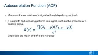
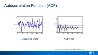
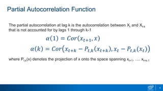
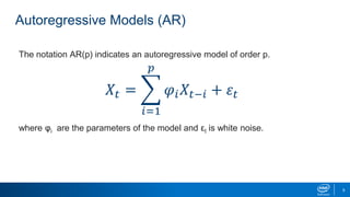
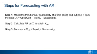
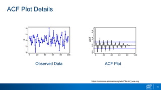
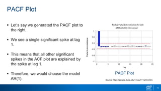
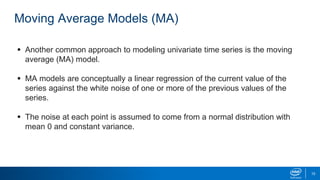
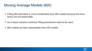
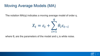
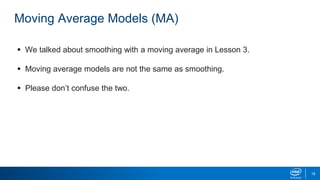
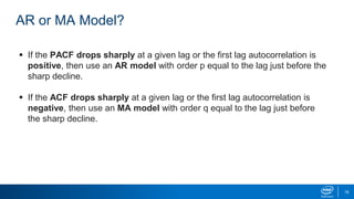
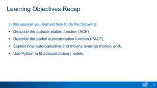
Lesson 4: AR-MA
1
Learning Objectives
You will be able to do the following:
 Describe the autocorrelation function (ACF).
 Describe the partial autocorrelation function (PACF).
 Explain how autoregressive and moving average models work.
 Use Python* to fit autocorrelation models.
2
ACF and PACF
Autocorrelation Function (ACF)
 Measures the correlation of a signal with a delayed copy of itself.
 It is used to find repeating patterns in a signal, such as the presence of a
periodic signal.
where μ is the mean and σ2 is the variance
𝑅 𝜏 =
𝐸 𝑋𝑡 − 𝜇 𝑋𝑡+𝜏 − 𝜇
𝜎2
4
Autocorrelation Function (ACF)
Observed Data ACF Plot
5
https://commons.wikimedia.org/wiki/File:Acf_new.svg
Partial Autocorrelation Function
The partial autocorrelation at lag k is the autocorrelation between Xt and Xt-k
that is not accounted for by lags 1 through k-1
where Pt,k(x) denotes the projection of x onto the space spanning xt+1, …. xt+k-1
𝛼 1 = 𝐶𝑜𝑟 𝑥 𝑡+1, 𝑥
𝛼 𝑘 = 𝐶𝑜𝑟 𝑥 𝑡+𝑘 − 𝑃𝑡,𝑘 𝑥 𝑡+𝑘 , 𝑥 𝑡 − 𝑃𝑡,𝑘(𝑥 𝑡)
6
Autoregressive Models
Autoregressive Models (AR)
 A common approach to model univariate time series is to use autoregressive
models (AR).
 An AR model is a linear regression of the current value of the series against
one or more prior values of the series.
 Uses maximum likelihood estimators to determine coefficients instead of
least squares.
8
Autoregressive Models (AR)
The notation AR(p) indicates an autoregressive model of order p.
where φi are the parameters of the model and εt is white noise.
𝑋𝑡 =
𝑖=1
𝑝
𝜑𝑖 𝑋𝑡−𝑖 + 𝜀𝑡
9
Autoregressive Models (AR)
 Useful for short term forecasts
 This model can forecast up to p values
10
Steps for Forecasting with AR
Step 1: Model the trend and/or seasonality of a time series and subtract it from
the data (Xt = Observedt – Trendt – Seasonalityt)
Step 2: Calculate AR on Xt to obtain Xt+1
Step 3: Forecast = Xt+1 + Trendt + Seasonalityt
11
ACF Plot Details
Observed Data ACF Plot
12
https://commons.wikimedia.org/wiki/File:Acf_new.svg
PACF Plot
PACF Plot
 Let’s say we generated the PACF plot to
the right.
 We see a single significant spike at lag
1.
 This means that all other significant
spikes in the ACF plot are explained by
the spike at lag 1.
 Therefore, we would choose the model
AR(1).
13
Source: https://people.duke.edu/~rnau/411arim3.htm
Moving Average Models
Moving Average Models (MA)
 Another common approach to modeling univariate time series is the moving
average (MA) model.
 MA models are conceptually a linear regression of the current value of the
series against the white noise of one or more of the previous values of the
series.
 The noise at each point is assumed to come from a normal distribution with
mean 0 and constant variance.
15
Moving Average Models (MA)
 Fitting MA estimates is more complicated than AR models because the error
terms are not observable.
 As a result, iterative nonlinear fitting procedures need to be used.
 MA models are less interpretable than AR models.
16
Moving Average Models (MA)
The notation MA(q) indicates a moving average model of order q.
where θi are the parameters of the model and εt is white noise.
𝑋𝑡 = 𝜀𝑡 +
𝑖=1
𝑞
𝜃𝑖 𝜀𝑡−𝑖
17
Moving Average Models (MA)
 We talked about smoothing with a moving average in Lesson 3.
 Moving average models are not the same as smoothing.
 Please don’t confuse the two.
18
AR or MA Model?
 If the PACF drops sharply at a given lag or the first lag autocorrelation is
positive, then use an AR model with order p equal to the lag just before the
sharp decline.
 If the ACF drops sharply at a given lag or the first lag autocorrelation is
negative, then use an MA model with order q equal to the lag just before
the sharp decline.
19
Applications in Python
Use Python to Fit Autocorrelation Models
Next up is a look at applying these concepts in Python.
 See notebook entitled Autocorrelation_student.ipynb
21
Learning Objectives Recap
In this session you learned how to do the following:
 Describe the autocorrelation function (ACF)
 Describe the partial autocorrelation function (PACF).
 Explain how autoregressive and moving average models work.
 Use Python to fit autocorrelation models.
22
Legal Notices and Disclaimers
This presentation is for informational purposes only. INTEL MAKES NO WARRANTIES, EXPRESS OR IMPLIED, IN THIS
SUMMARY.
Intel technologies’ features and benefits depend on system configuration and may require enabled hardware, software or
service activation. Performance varies depending on system configuration. Check with your system manufacturer or
retailer or learn more at intel.com.
Sample source code is released under the Intel Sample Source Code License Agreement.
Intel, the Intel logo, the Intel. Experience What’s Inside logo, and Intel. Experience What’s Inside are trademarks of Intel
Corporation in the U.S. and/or other countries.
*Other names and brands may be claimed as the property of others.
Copyright © 2018, Intel Corporation. All rights reserved.
23
Lesson 4 ar-ma

Lesson 4 ar-ma

  • 1.
  • 2.
    Learning Objectives You willbe able to do the following:  Describe the autocorrelation function (ACF).  Describe the partial autocorrelation function (PACF).  Explain how autoregressive and moving average models work.  Use Python* to fit autocorrelation models. 2
  • 3.
  • 4.
    Autocorrelation Function (ACF) Measures the correlation of a signal with a delayed copy of itself.  It is used to find repeating patterns in a signal, such as the presence of a periodic signal. where μ is the mean and σ2 is the variance 𝑅 𝜏 = 𝐸 𝑋𝑡 − 𝜇 𝑋𝑡+𝜏 − 𝜇 𝜎2 4
  • 5.
    Autocorrelation Function (ACF) ObservedData ACF Plot 5 https://commons.wikimedia.org/wiki/File:Acf_new.svg
  • 6.
    Partial Autocorrelation Function Thepartial autocorrelation at lag k is the autocorrelation between Xt and Xt-k that is not accounted for by lags 1 through k-1 where Pt,k(x) denotes the projection of x onto the space spanning xt+1, …. xt+k-1 𝛼 1 = 𝐶𝑜𝑟 𝑥 𝑡+1, 𝑥 𝛼 𝑘 = 𝐶𝑜𝑟 𝑥 𝑡+𝑘 − 𝑃𝑡,𝑘 𝑥 𝑡+𝑘 , 𝑥 𝑡 − 𝑃𝑡,𝑘(𝑥 𝑡) 6
  • 7.
  • 8.
    Autoregressive Models (AR) A common approach to model univariate time series is to use autoregressive models (AR).  An AR model is a linear regression of the current value of the series against one or more prior values of the series.  Uses maximum likelihood estimators to determine coefficients instead of least squares. 8
  • 9.
    Autoregressive Models (AR) Thenotation AR(p) indicates an autoregressive model of order p. where φi are the parameters of the model and εt is white noise. 𝑋𝑡 = 𝑖=1 𝑝 𝜑𝑖 𝑋𝑡−𝑖 + 𝜀𝑡 9
  • 10.
    Autoregressive Models (AR) Useful for short term forecasts  This model can forecast up to p values 10
  • 11.
    Steps for Forecastingwith AR Step 1: Model the trend and/or seasonality of a time series and subtract it from the data (Xt = Observedt – Trendt – Seasonalityt) Step 2: Calculate AR on Xt to obtain Xt+1 Step 3: Forecast = Xt+1 + Trendt + Seasonalityt 11
  • 12.
    ACF Plot Details ObservedData ACF Plot 12 https://commons.wikimedia.org/wiki/File:Acf_new.svg
  • 13.
    PACF Plot PACF Plot Let’s say we generated the PACF plot to the right.  We see a single significant spike at lag 1.  This means that all other significant spikes in the ACF plot are explained by the spike at lag 1.  Therefore, we would choose the model AR(1). 13 Source: https://people.duke.edu/~rnau/411arim3.htm
  • 14.
  • 15.
    Moving Average Models(MA)  Another common approach to modeling univariate time series is the moving average (MA) model.  MA models are conceptually a linear regression of the current value of the series against the white noise of one or more of the previous values of the series.  The noise at each point is assumed to come from a normal distribution with mean 0 and constant variance. 15
  • 16.
    Moving Average Models(MA)  Fitting MA estimates is more complicated than AR models because the error terms are not observable.  As a result, iterative nonlinear fitting procedures need to be used.  MA models are less interpretable than AR models. 16
  • 17.
    Moving Average Models(MA) The notation MA(q) indicates a moving average model of order q. where θi are the parameters of the model and εt is white noise. 𝑋𝑡 = 𝜀𝑡 + 𝑖=1 𝑞 𝜃𝑖 𝜀𝑡−𝑖 17
  • 18.
    Moving Average Models(MA)  We talked about smoothing with a moving average in Lesson 3.  Moving average models are not the same as smoothing.  Please don’t confuse the two. 18
  • 19.
    AR or MAModel?  If the PACF drops sharply at a given lag or the first lag autocorrelation is positive, then use an AR model with order p equal to the lag just before the sharp decline.  If the ACF drops sharply at a given lag or the first lag autocorrelation is negative, then use an MA model with order q equal to the lag just before the sharp decline. 19
  • 20.
  • 21.
    Use Python toFit Autocorrelation Models Next up is a look at applying these concepts in Python.  See notebook entitled Autocorrelation_student.ipynb 21
  • 22.
    Learning Objectives Recap Inthis session you learned how to do the following:  Describe the autocorrelation function (ACF)  Describe the partial autocorrelation function (PACF).  Explain how autoregressive and moving average models work.  Use Python to fit autocorrelation models. 22
  • 23.
    Legal Notices andDisclaimers This presentation is for informational purposes only. INTEL MAKES NO WARRANTIES, EXPRESS OR IMPLIED, IN THIS SUMMARY. Intel technologies’ features and benefits depend on system configuration and may require enabled hardware, software or service activation. Performance varies depending on system configuration. Check with your system manufacturer or retailer or learn more at intel.com. Sample source code is released under the Intel Sample Source Code License Agreement. Intel, the Intel logo, the Intel. Experience What’s Inside logo, and Intel. Experience What’s Inside are trademarks of Intel Corporation in the U.S. and/or other countries. *Other names and brands may be claimed as the property of others. Copyright © 2018, Intel Corporation. All rights reserved. 23