


![Use Case: Fit A Time Series Model
For instructor
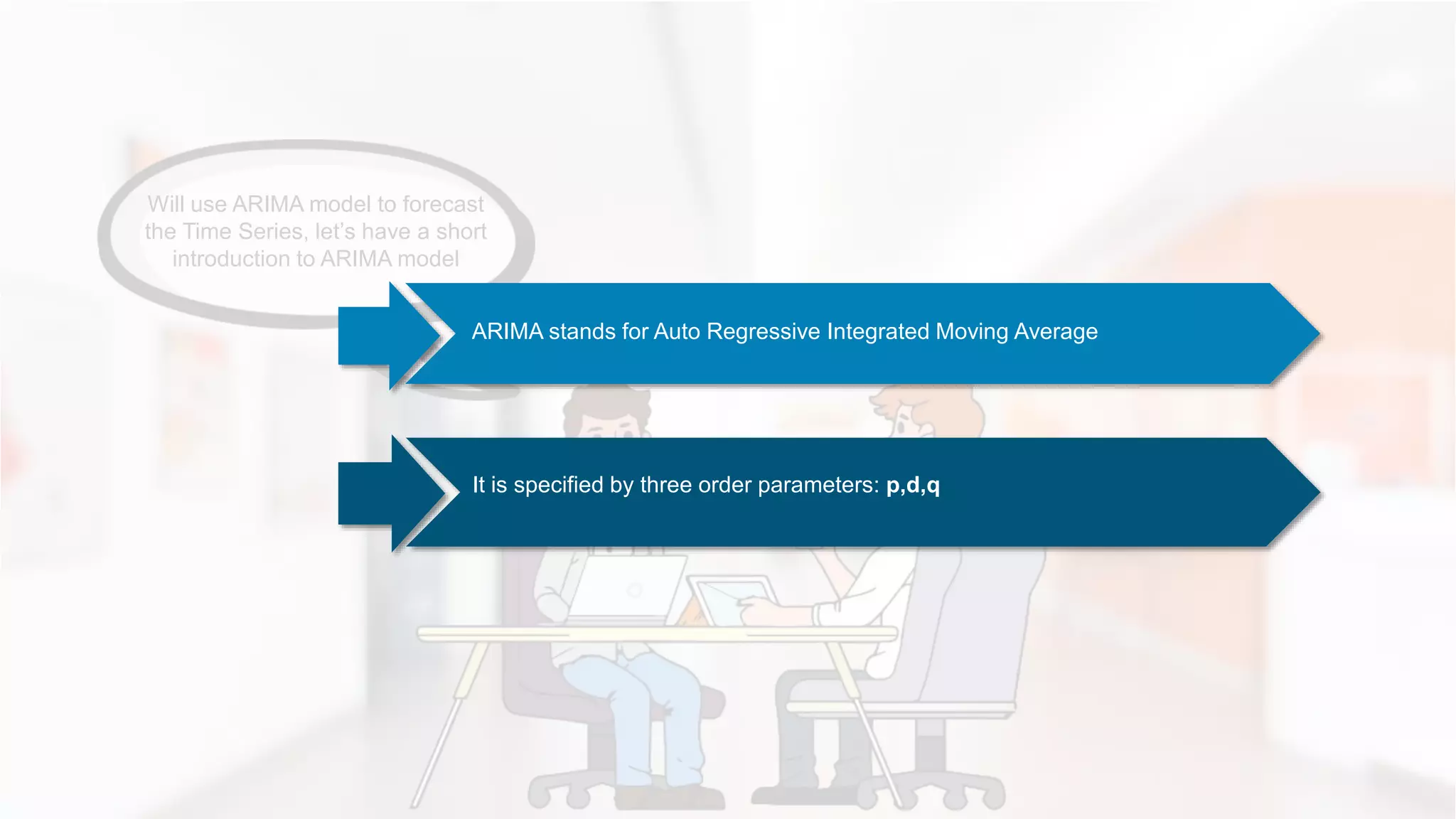
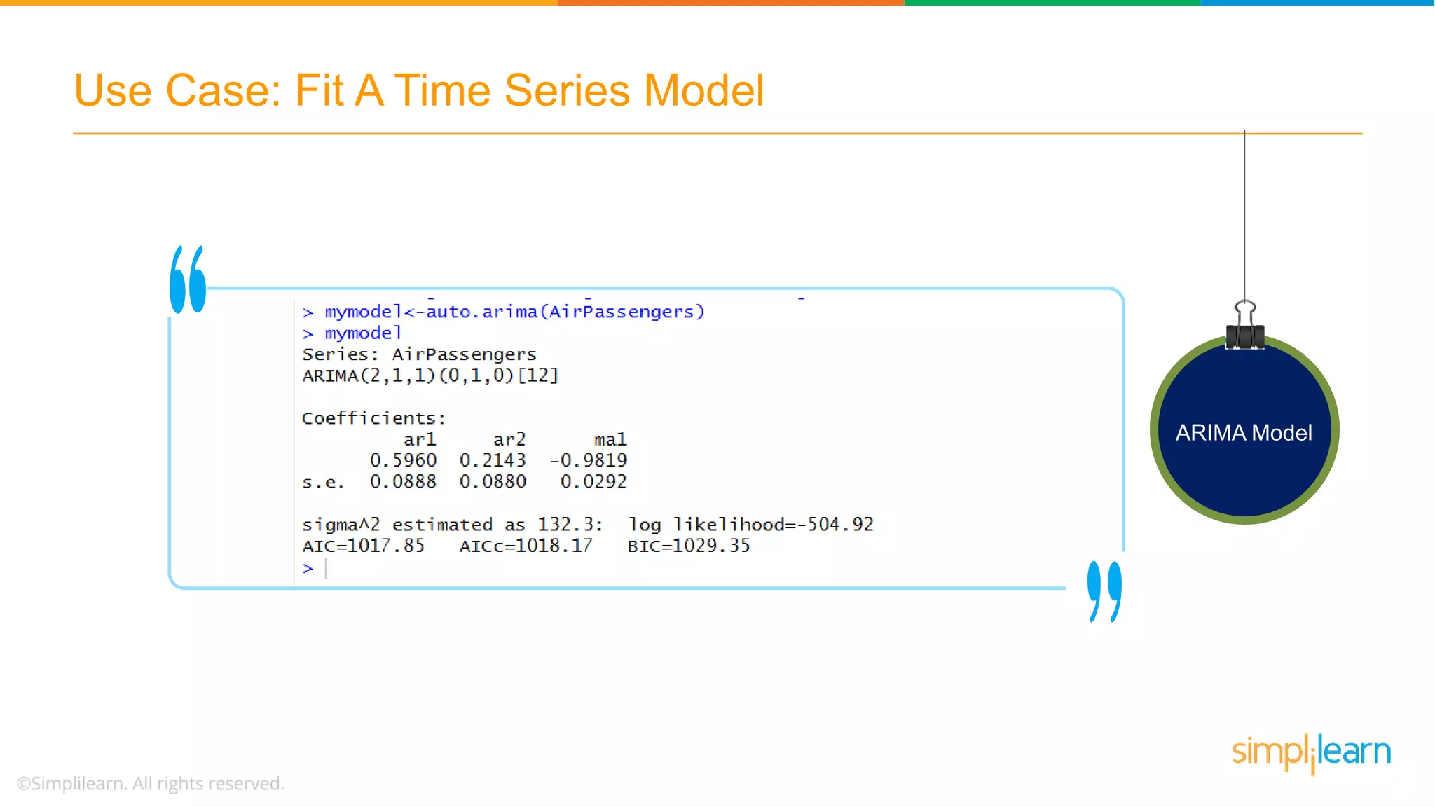
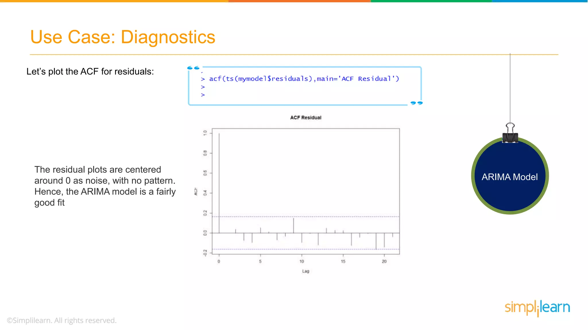
ARIMA Model
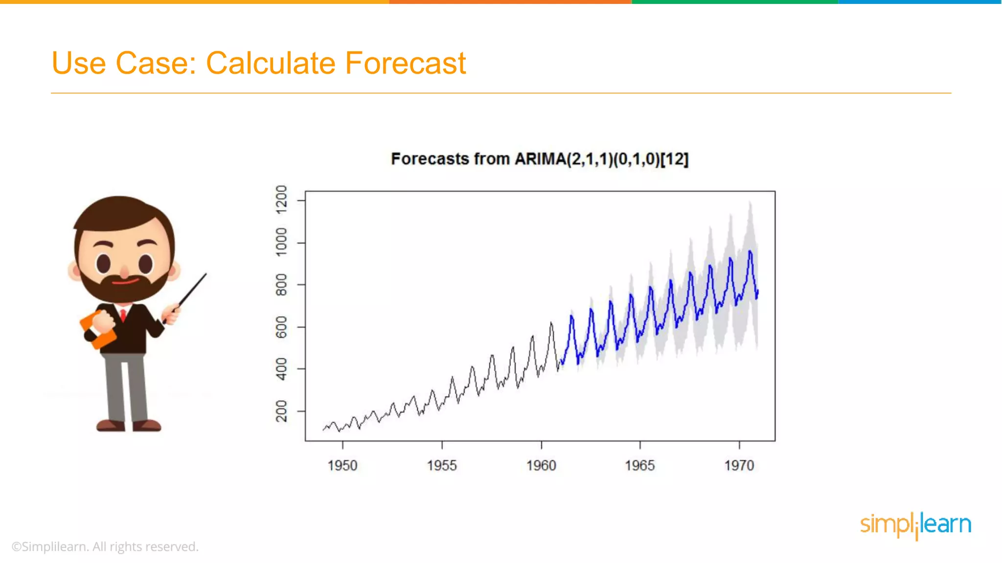
The ARIMA(2,1,1)(0,1,0)[12] model parameters are:
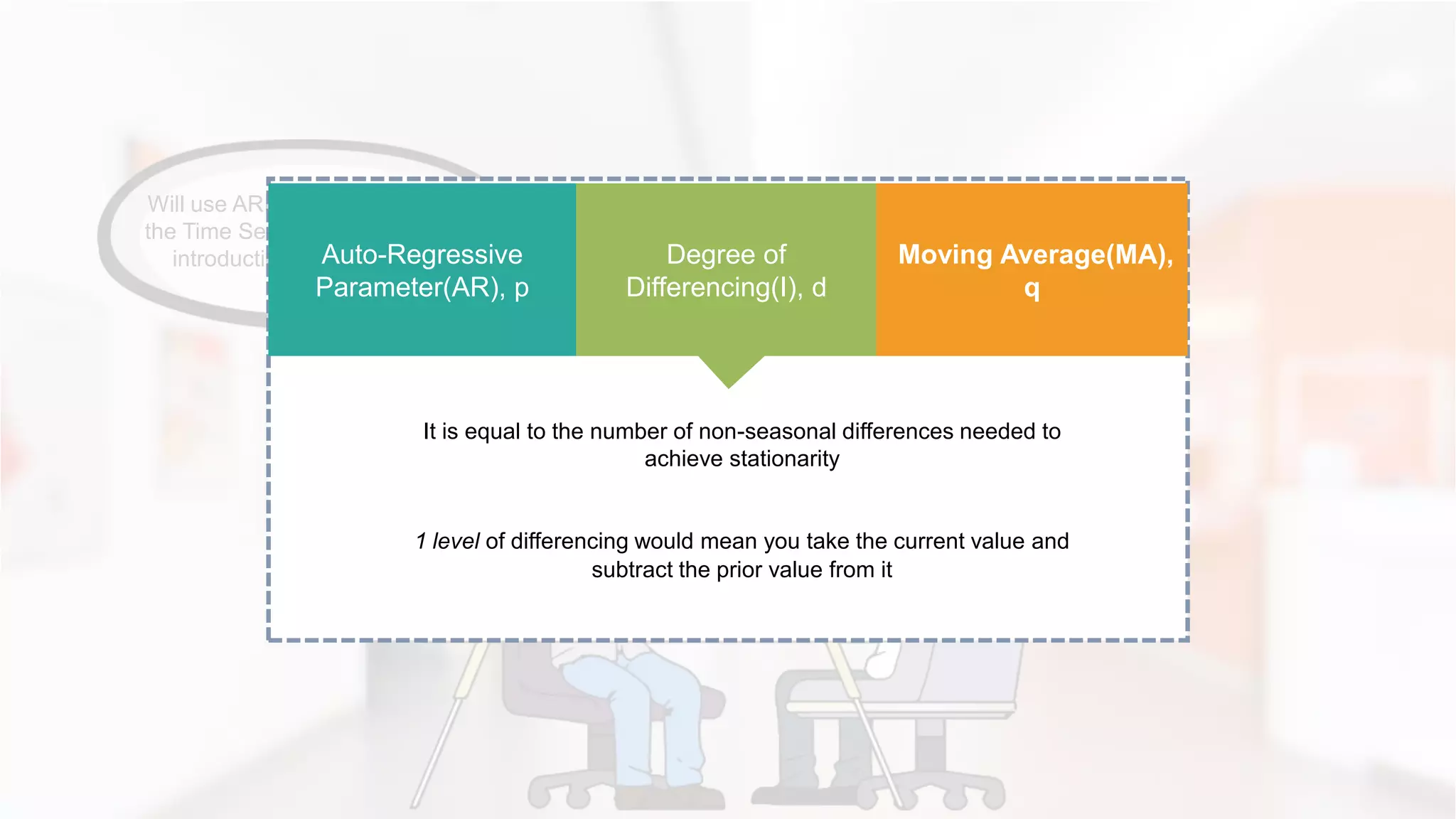
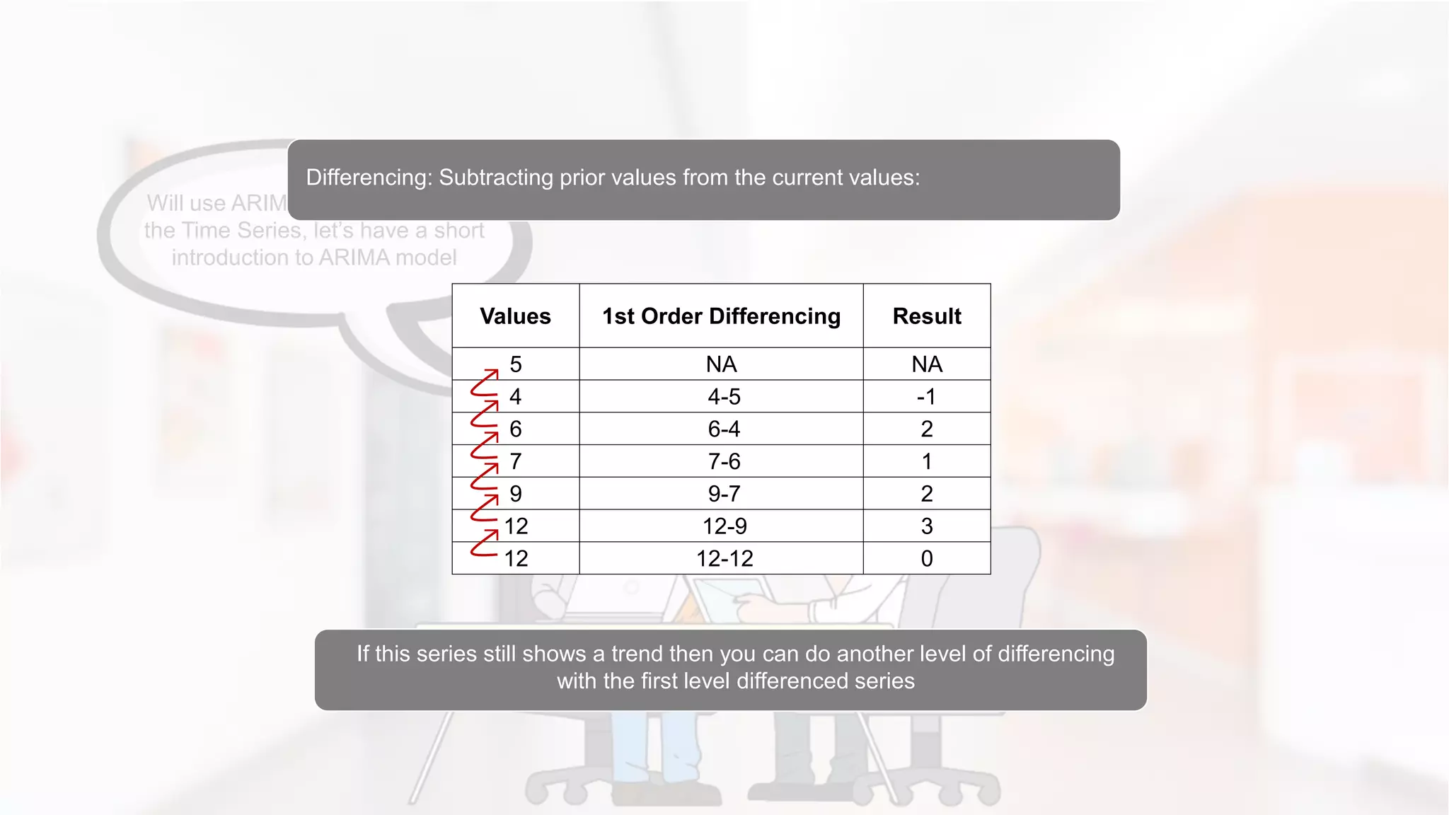
Lag 1 differencing (d),
An autoregressive term of second lag (p),
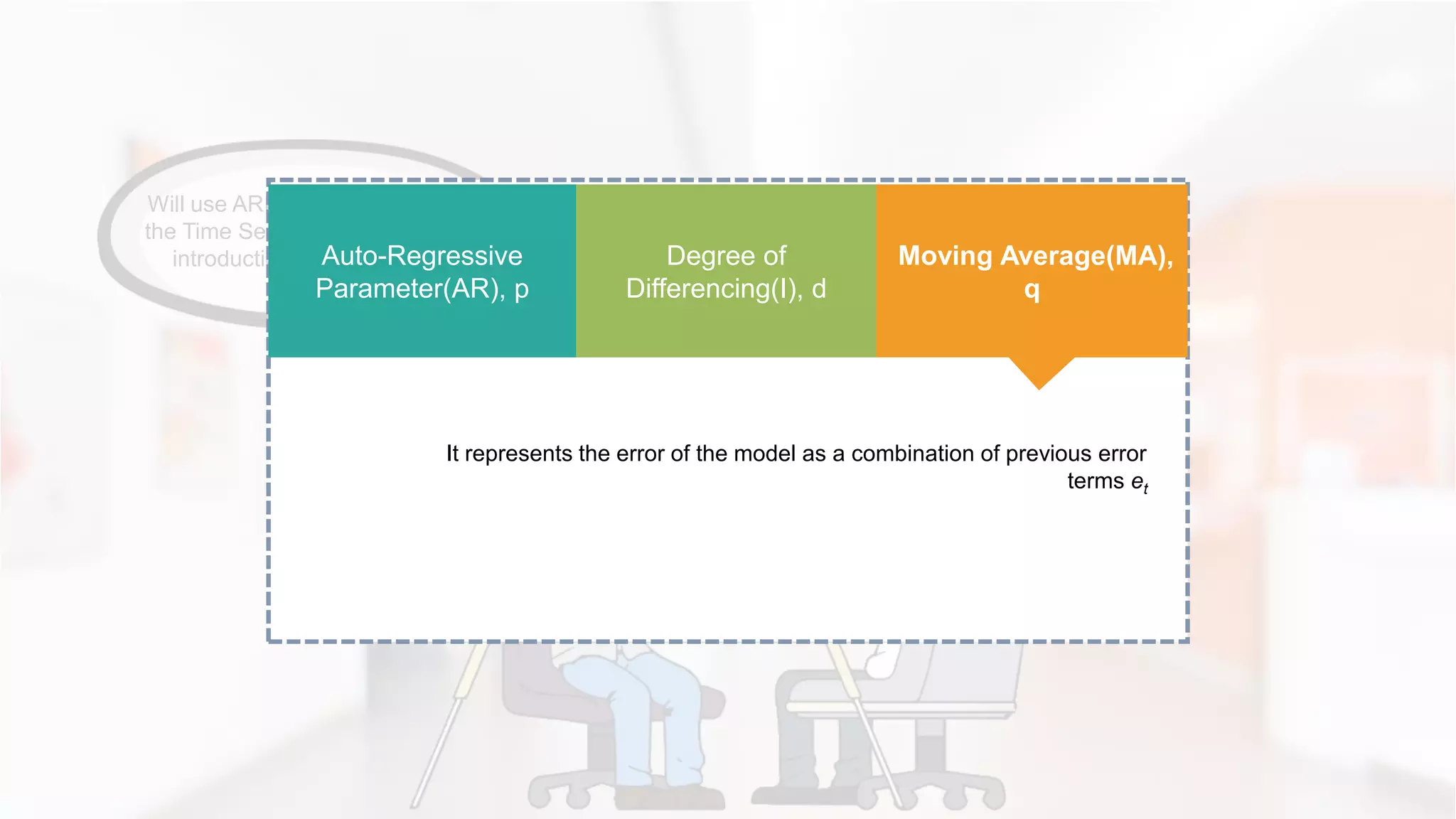
A moving average model of order 1 (q)
Then the seasonal model has an autoregressive term of first lag (D) at
model period 12 units, in this case months](https://image.slidesharecdn.com/timeseriesanalysis-2timeseriesinrarimamodelforecastingdatasciencesimplilearn-180705083509/75/Time-Series-Analysis-2-Time-Series-in-R-ARIMA-Model-Forecasting-Data-Science-Simplilearn-55-2048.jpg)


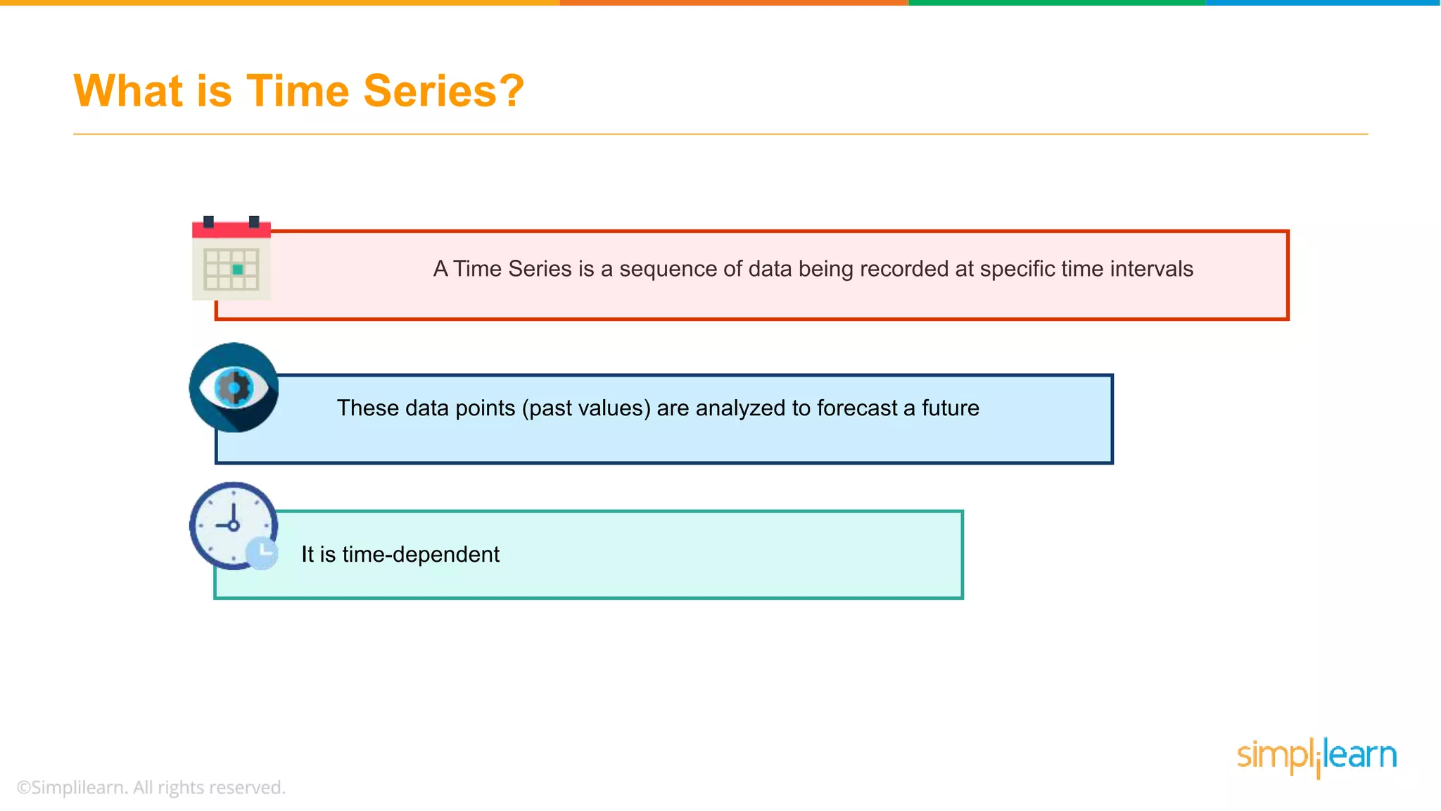
The document provides an overview of implementing time series analysis using R, focusing on concepts like stationarity, ARIMA models, and forecasting methodologies. It discusses the components of time series, the significance of autocorrelation, and the process of model validation through the Ljung-Box test. Additionally, it illustrates practical examples of forecasting air-ticket sales data and the decomposition of time series into trend, seasonality, and irregularity components.
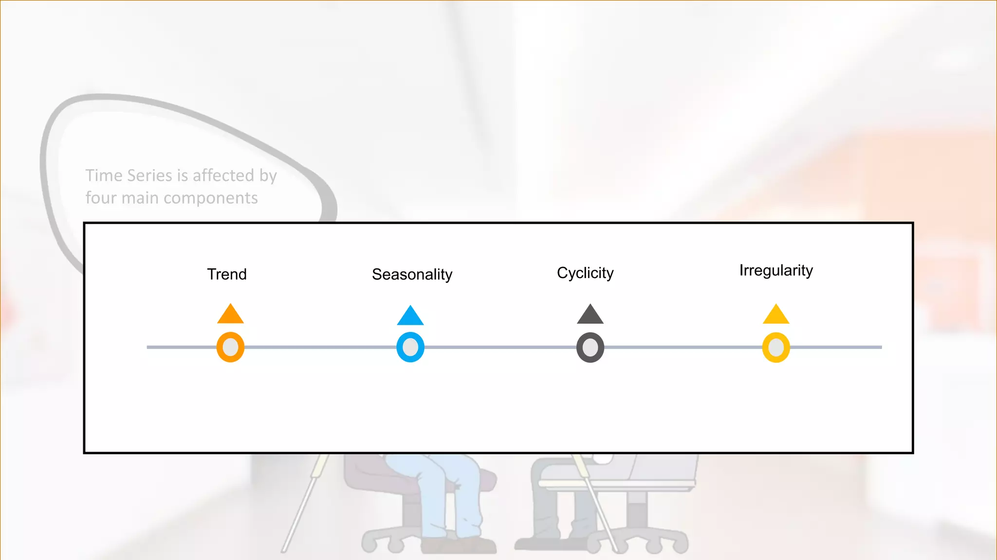
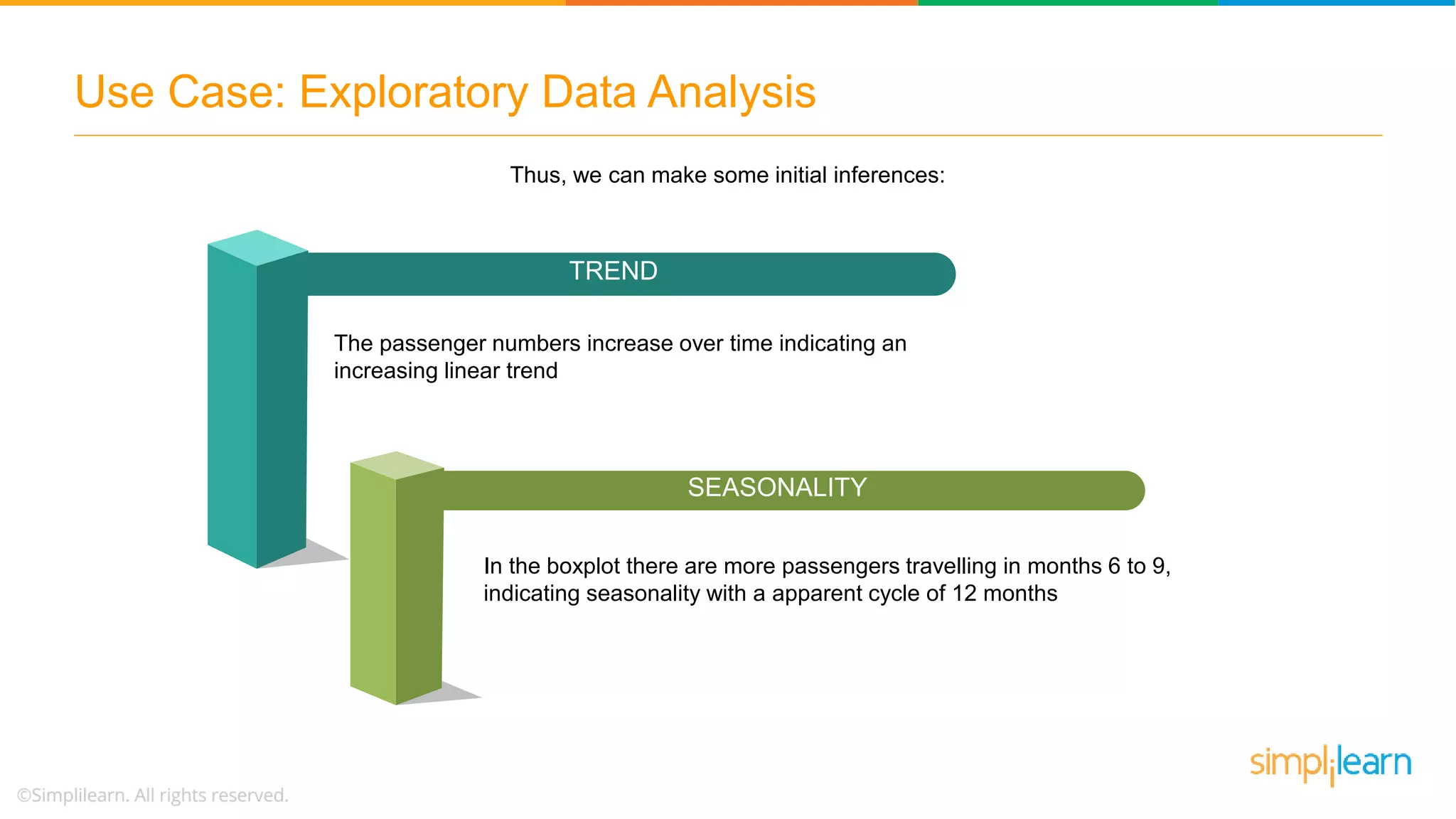
Overview of Time Series, its components (Trend, Seasonality, Cyclicity, Irregularity), and forecasting principles.
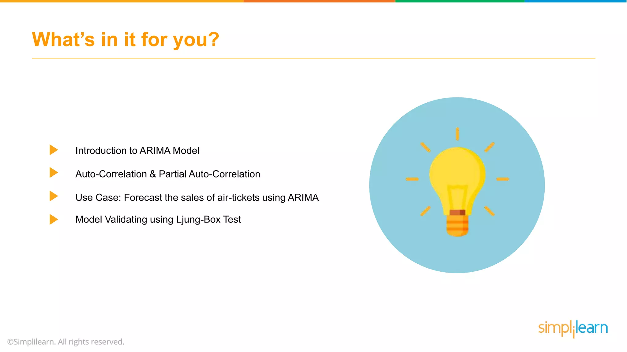
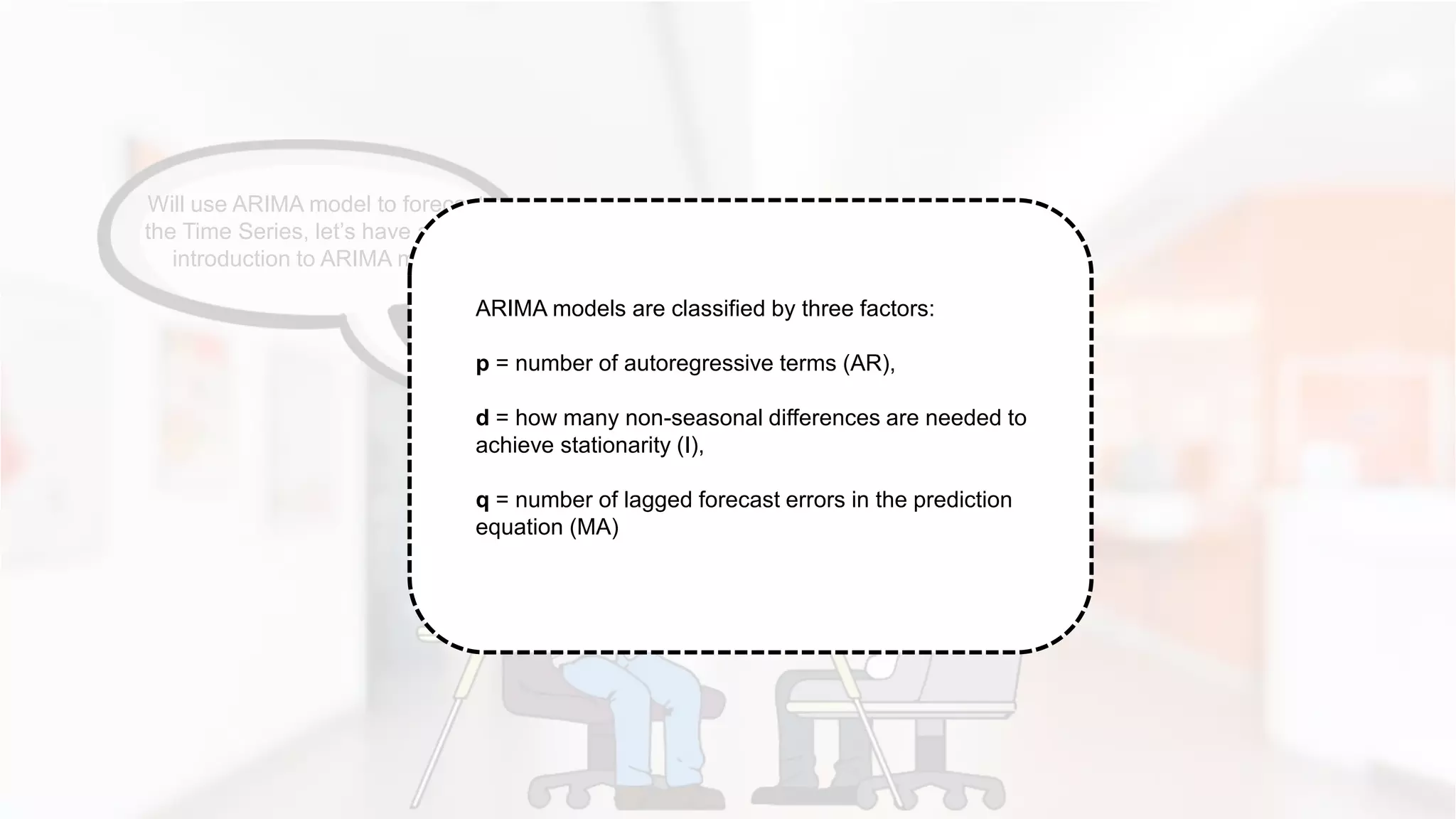
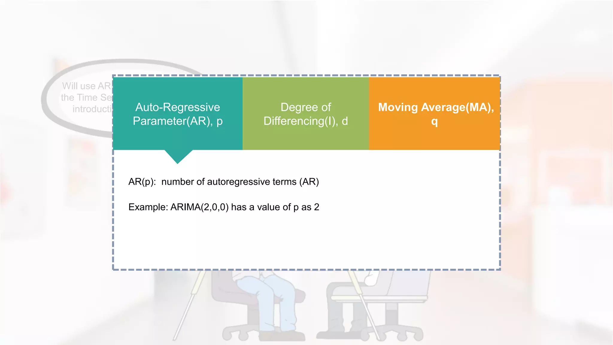
Introduction to ARIMA model, explaining its parameters (p, d, q) and significance in forecasting Time Series.
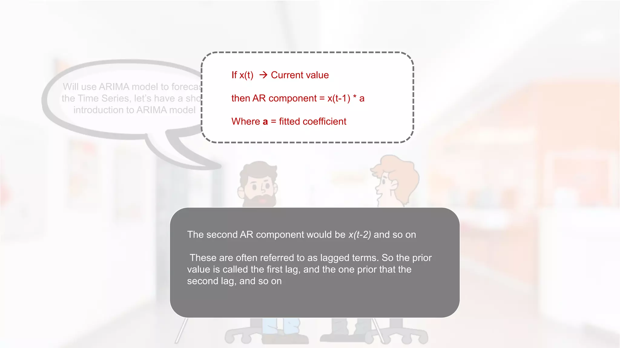
Detailed explanation of autoregressive (AR) terms and their role in Time Series modeling.
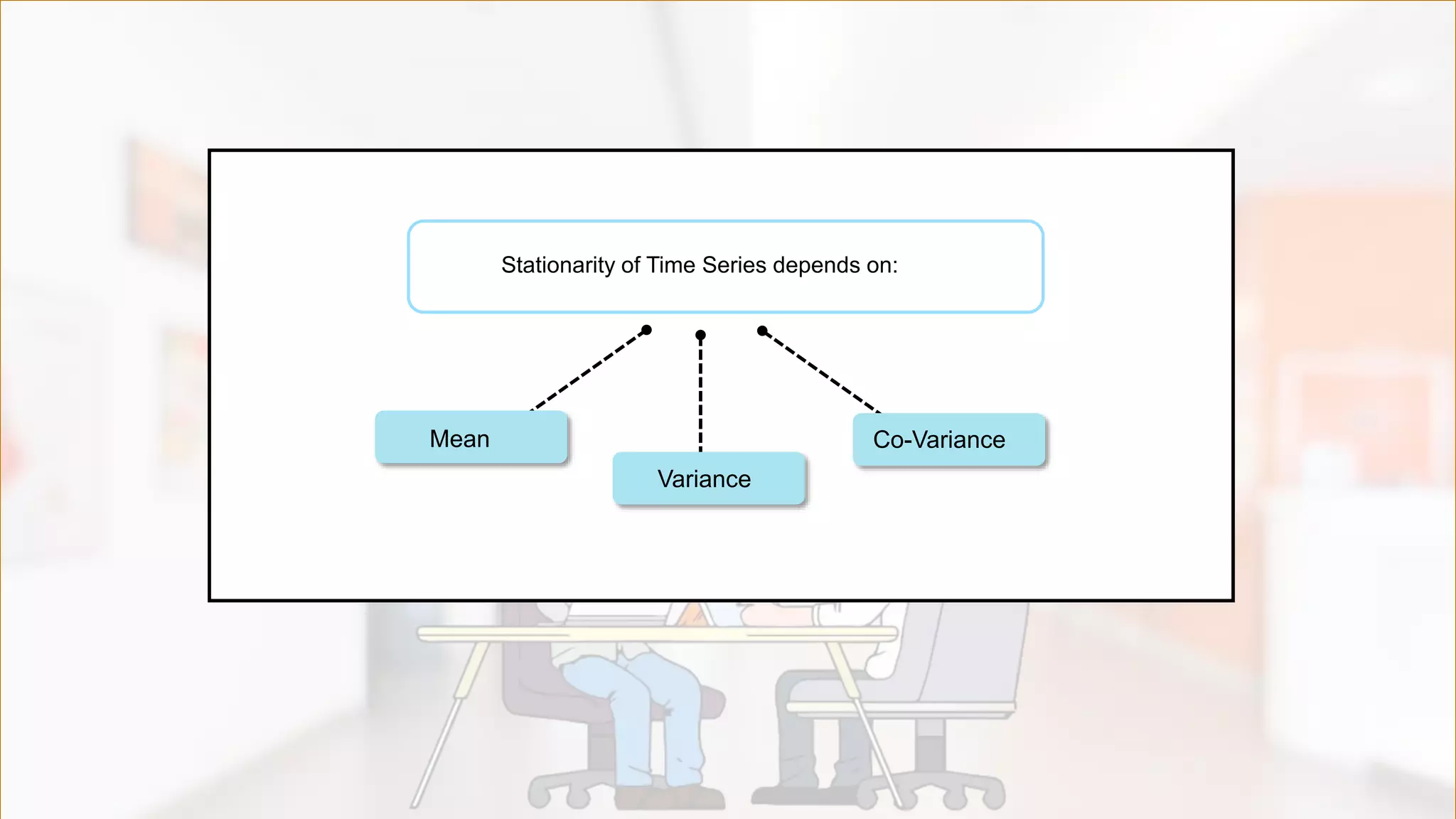
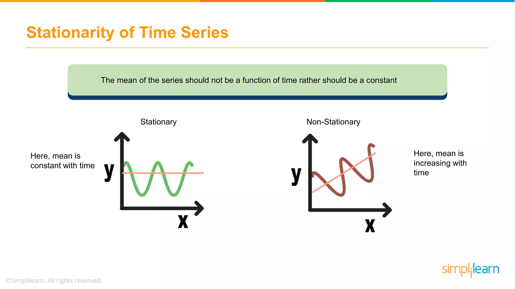
Importance of stationarity in Time Series, specifically discussing trends and seasonality.
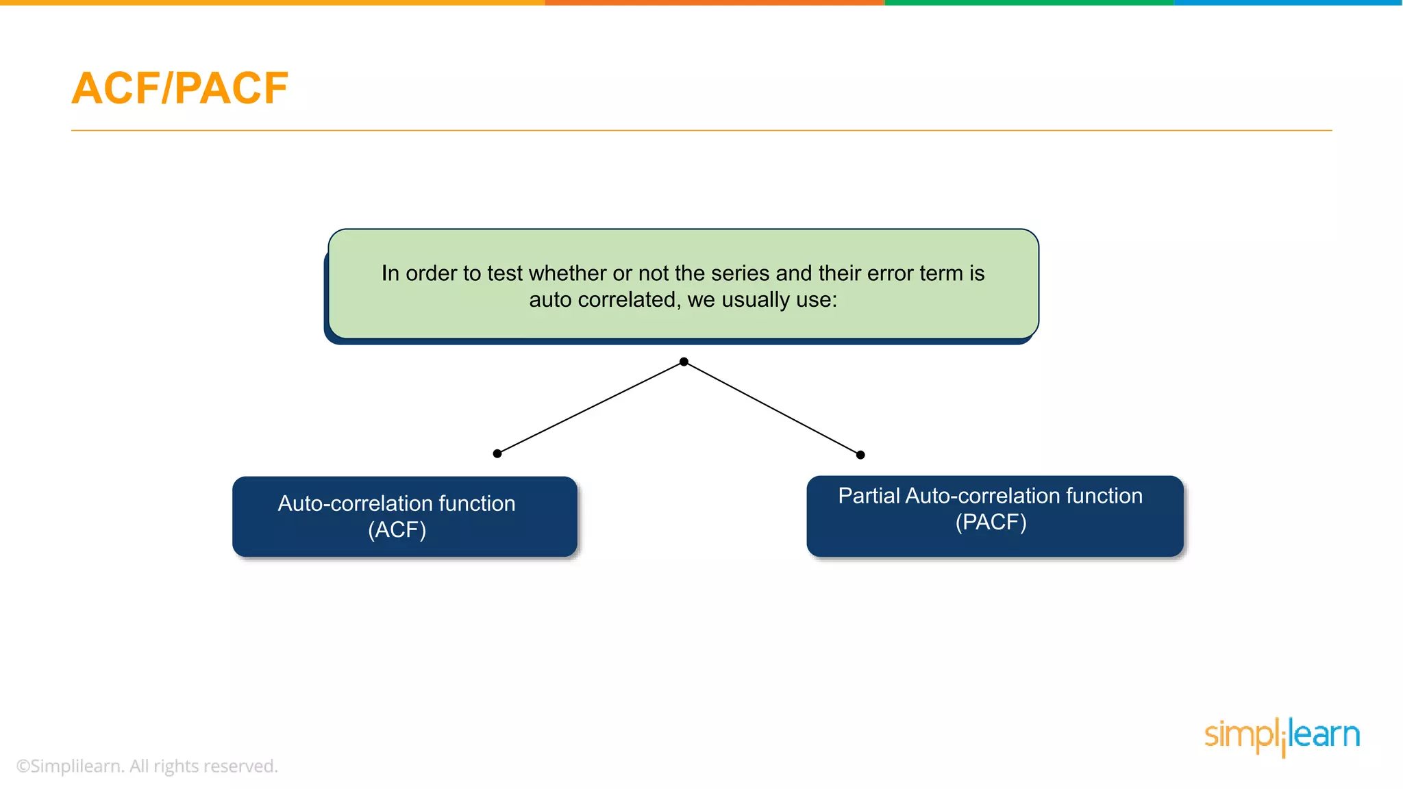
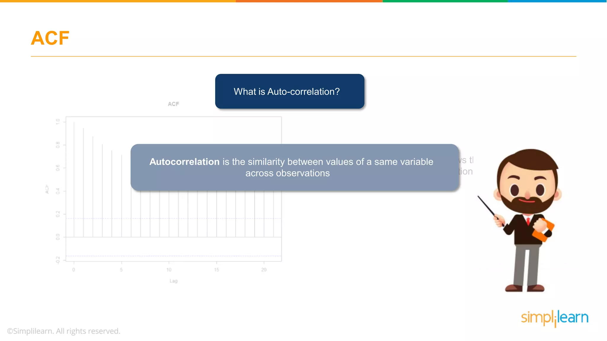
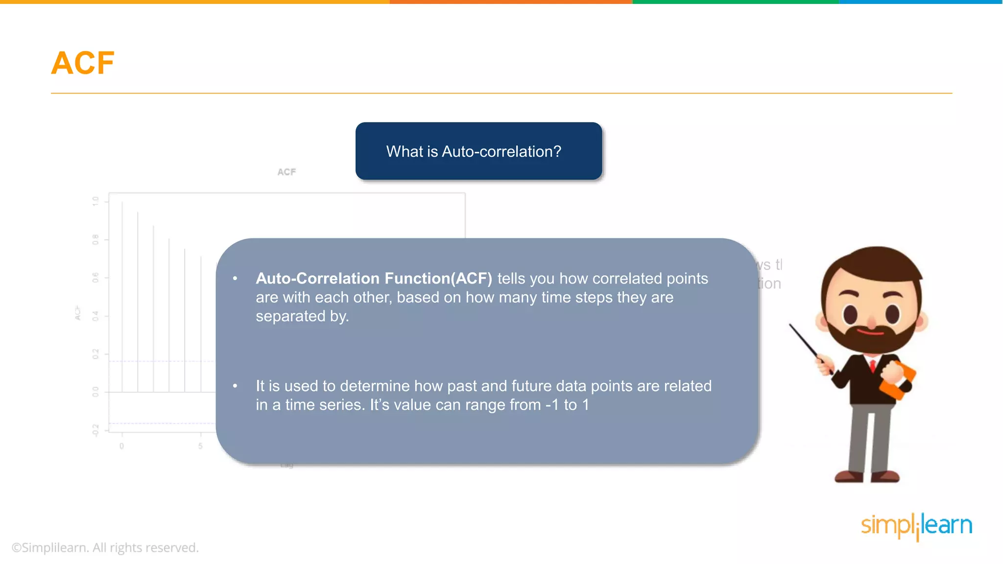
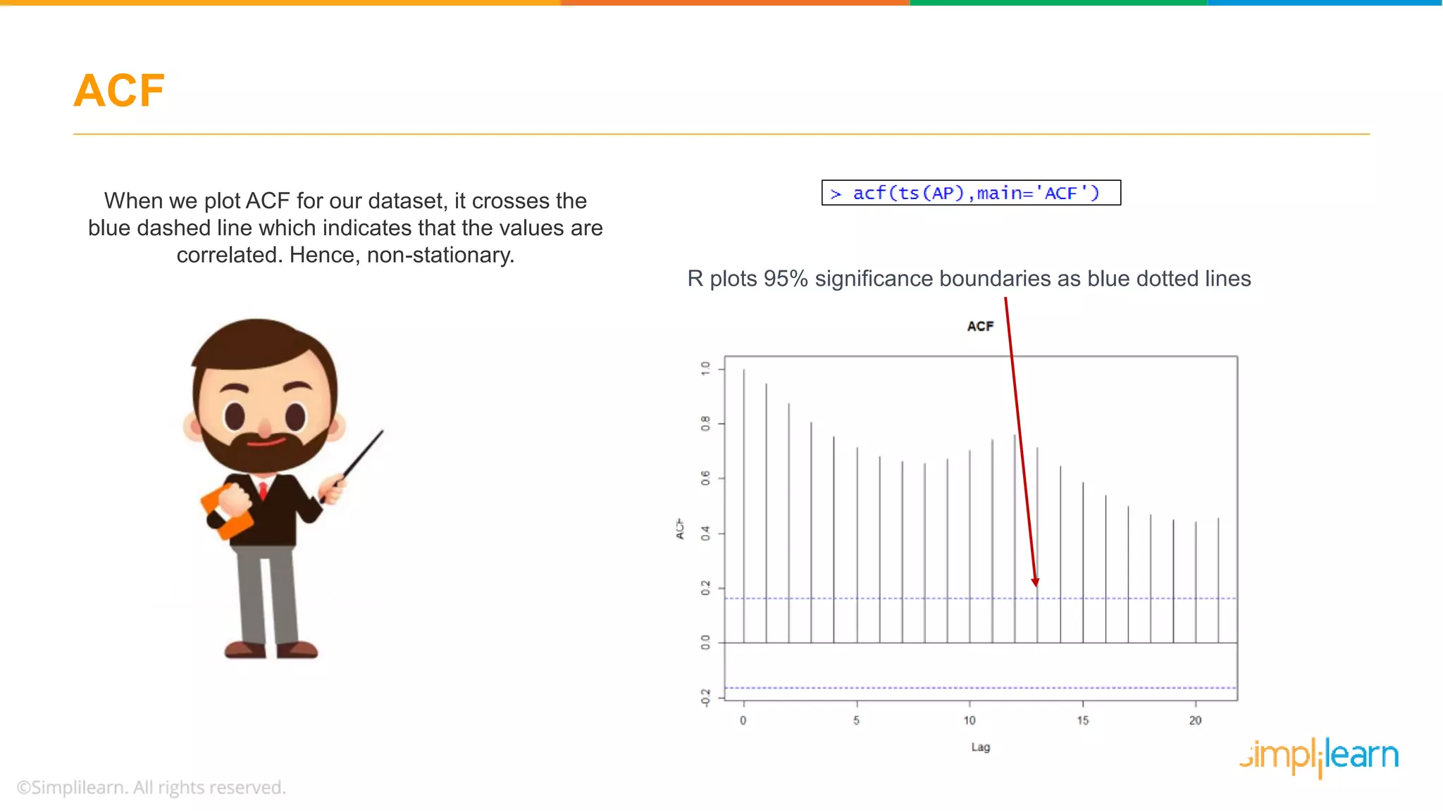
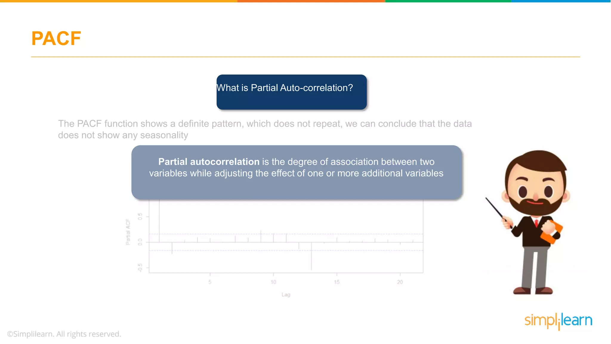
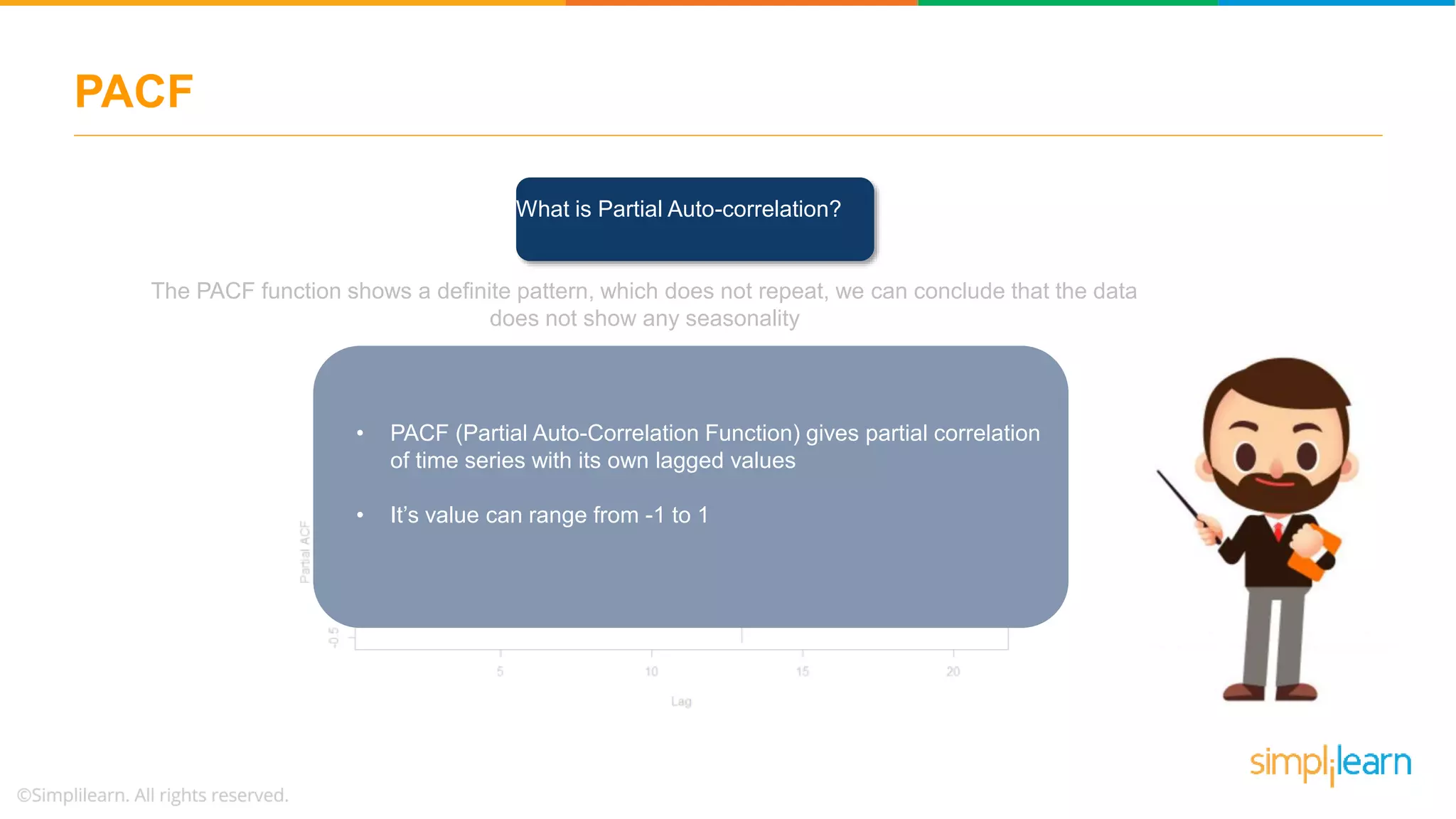
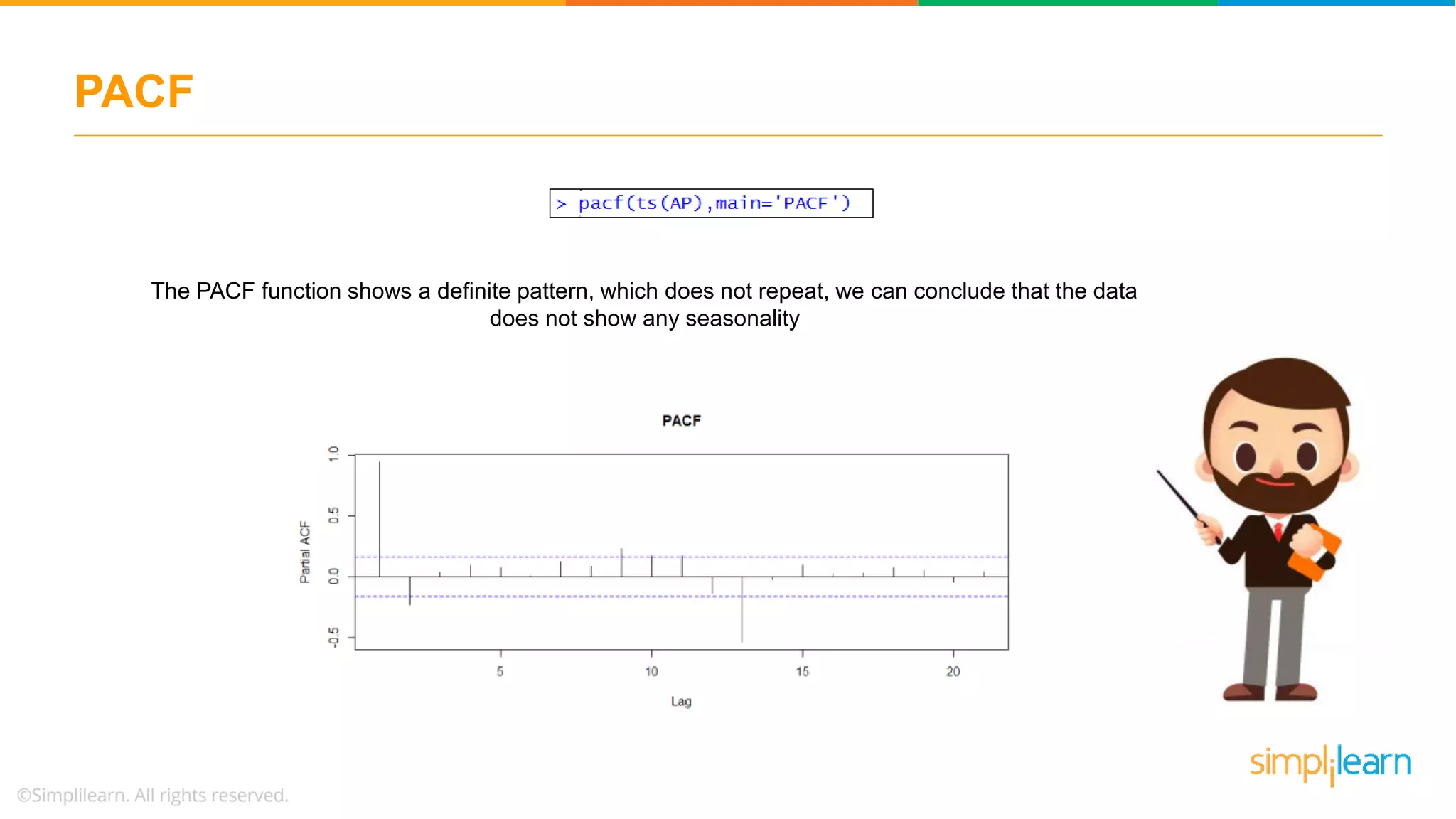
Introduction to Auto-Correlation Function (ACF) and Partial Auto-Correlation Function (PACF) used for diagnosing Time Series data.
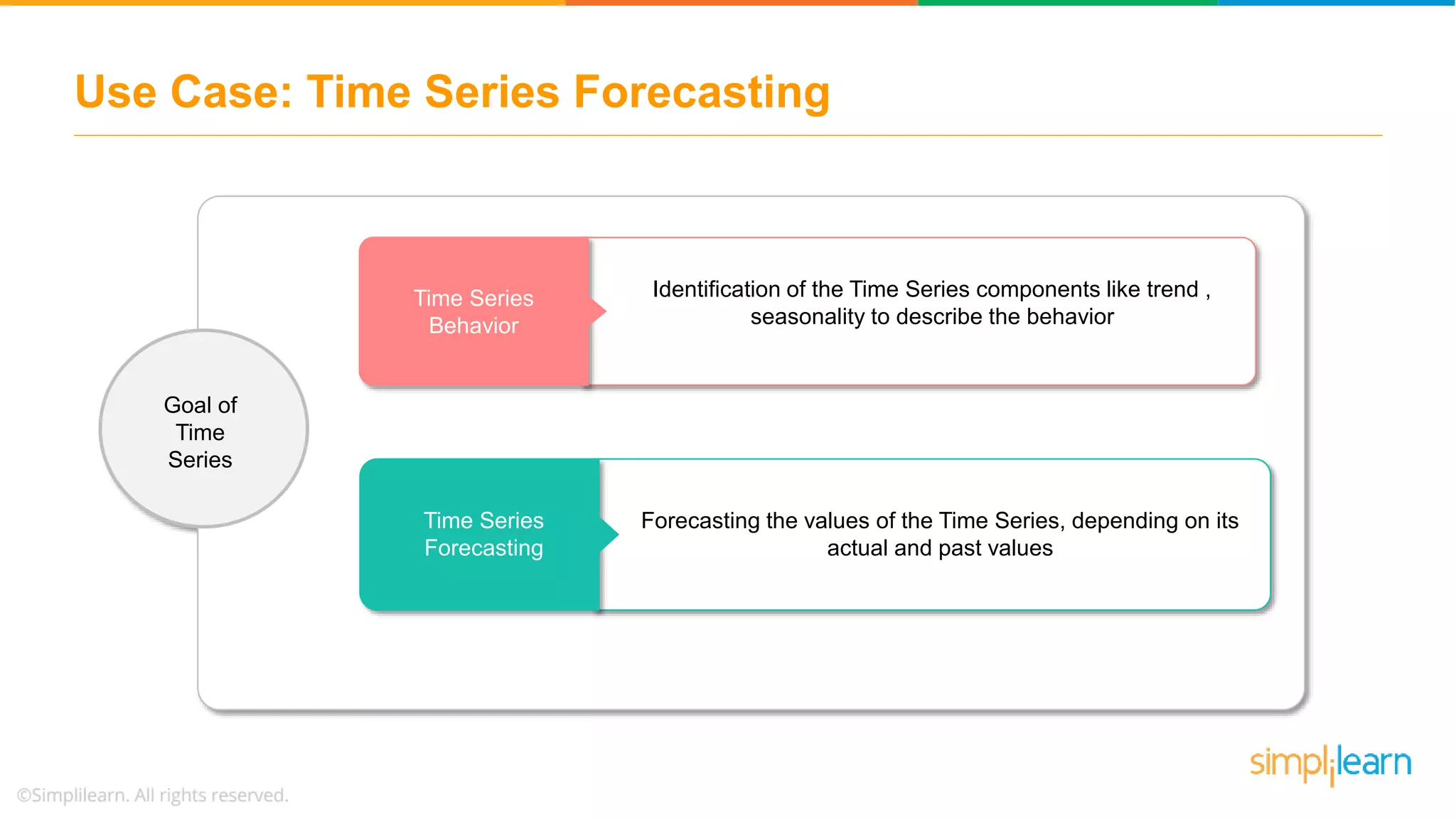
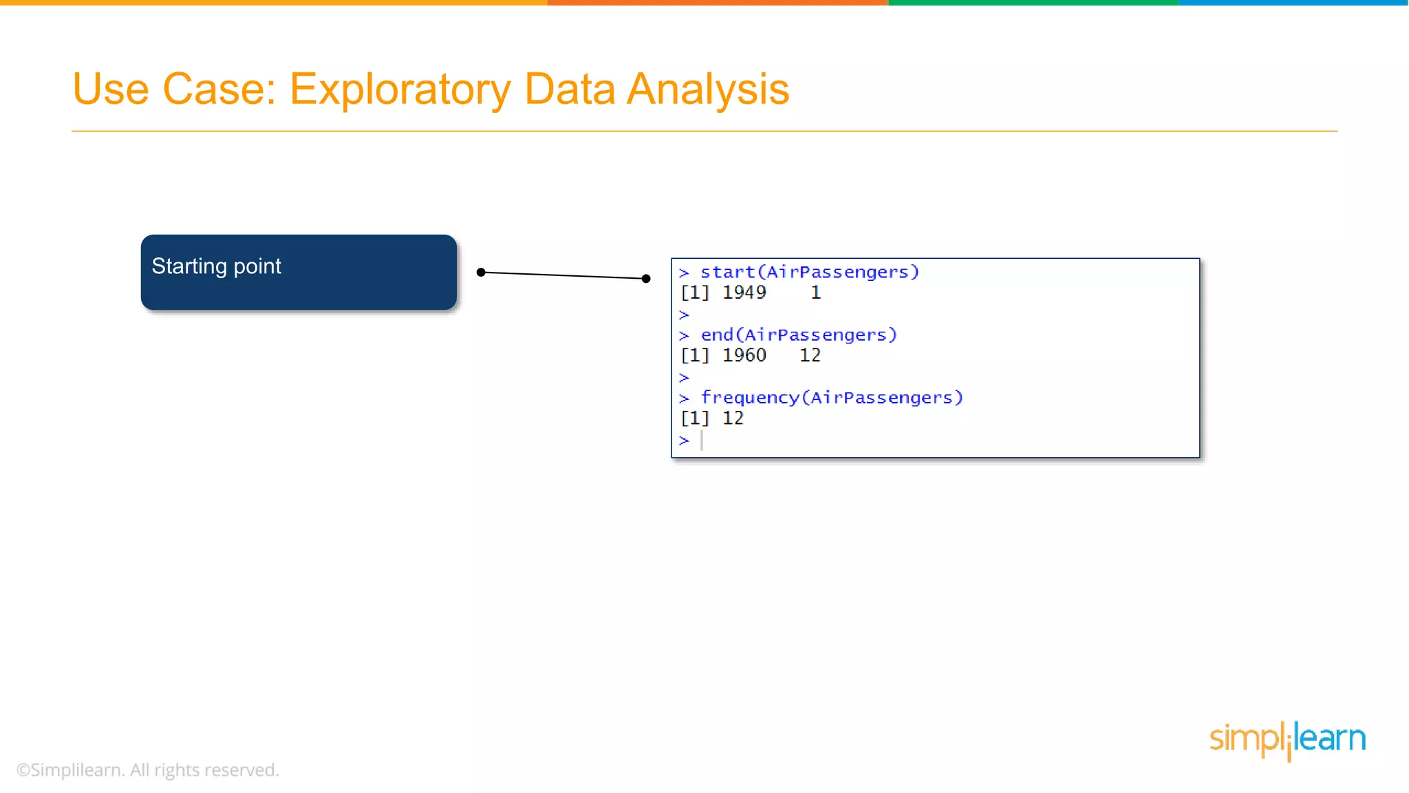
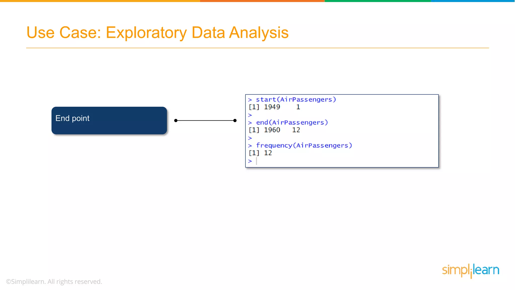
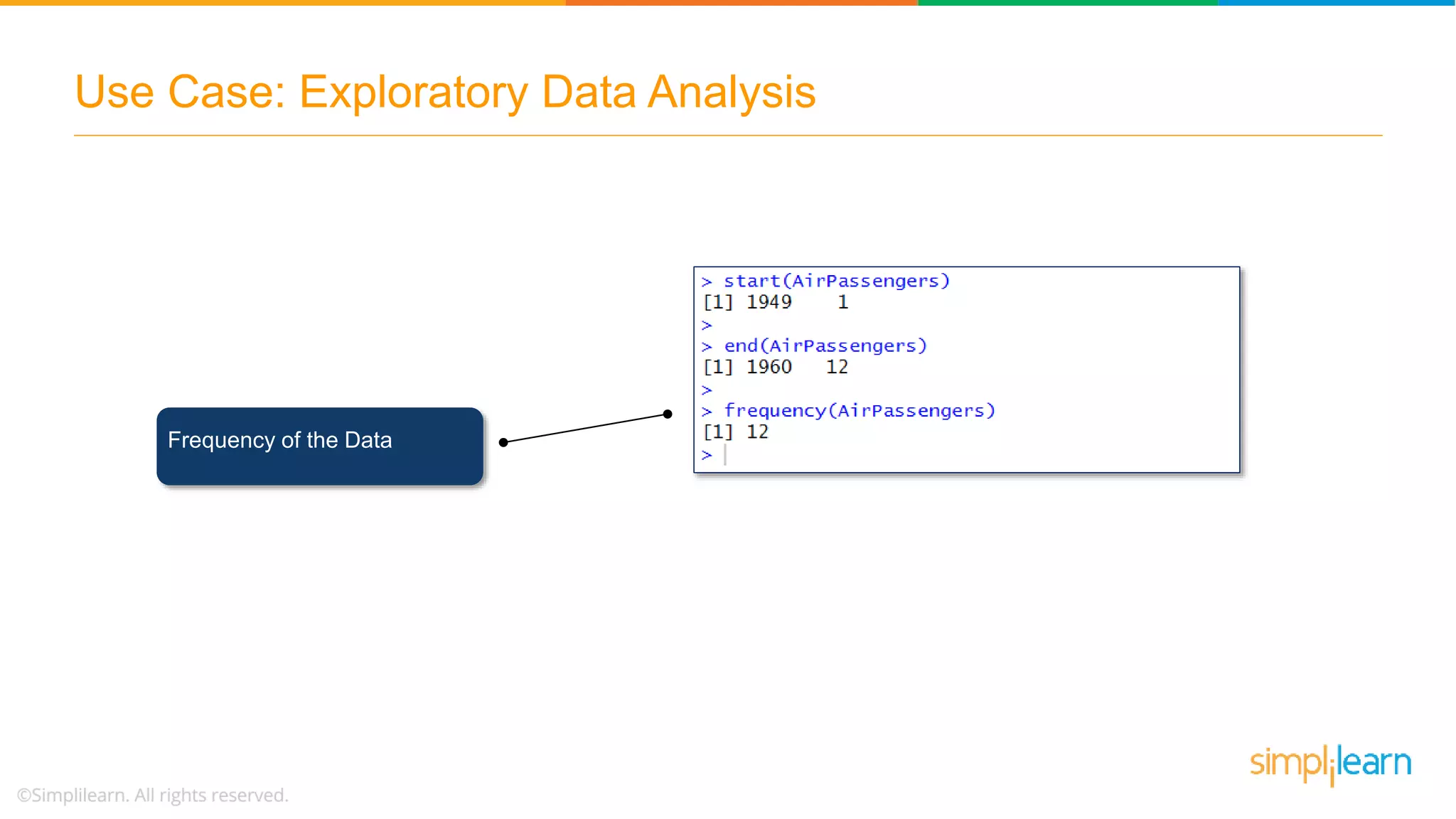
A practical example forecasting airline ticket sales using a 10-year dataset, emphasizing the Time Series behavior.
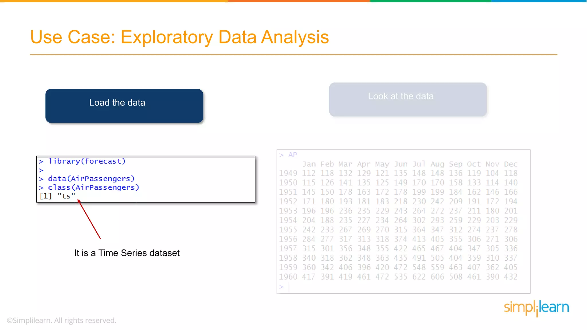
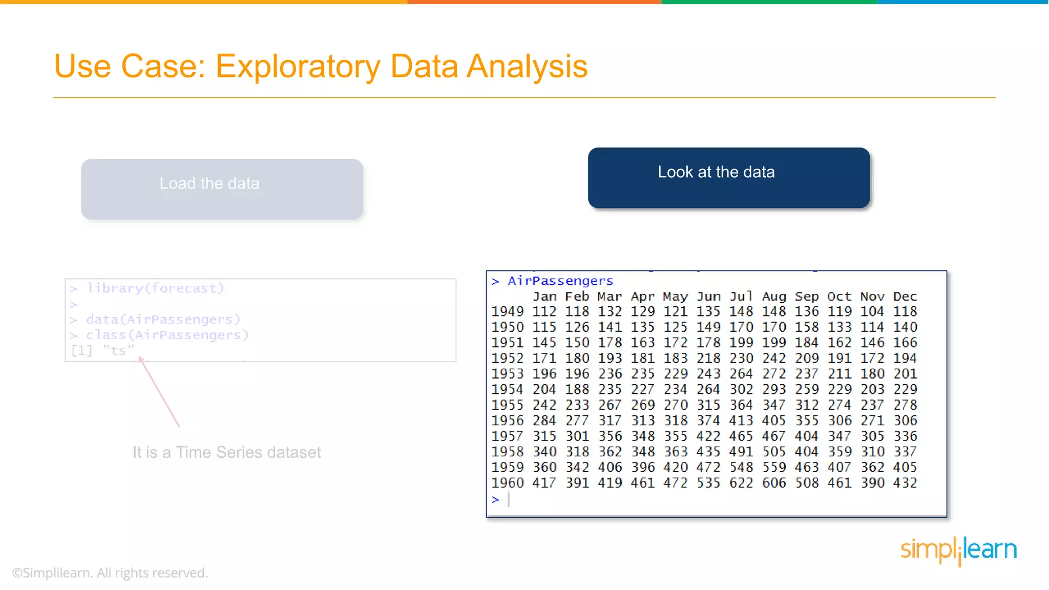
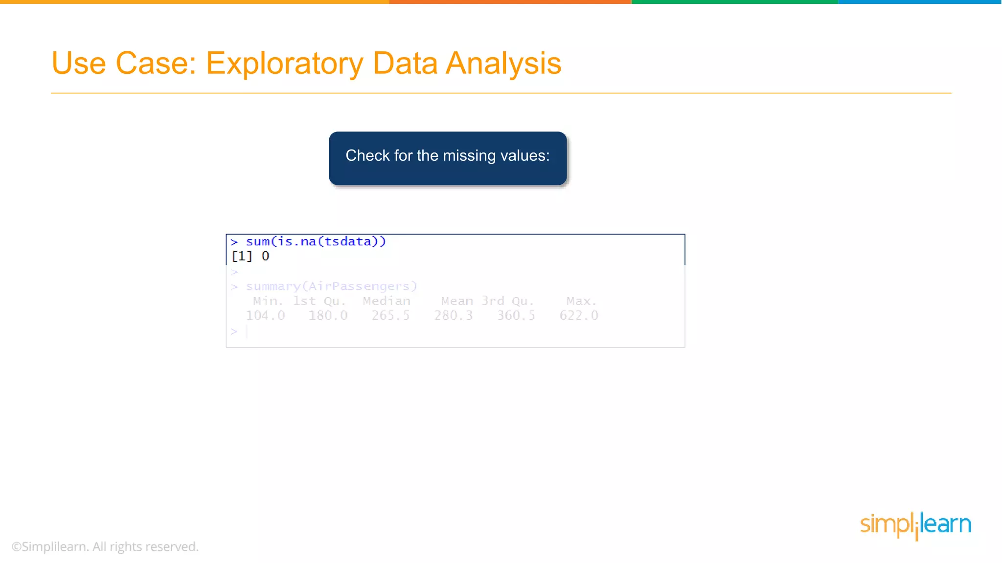
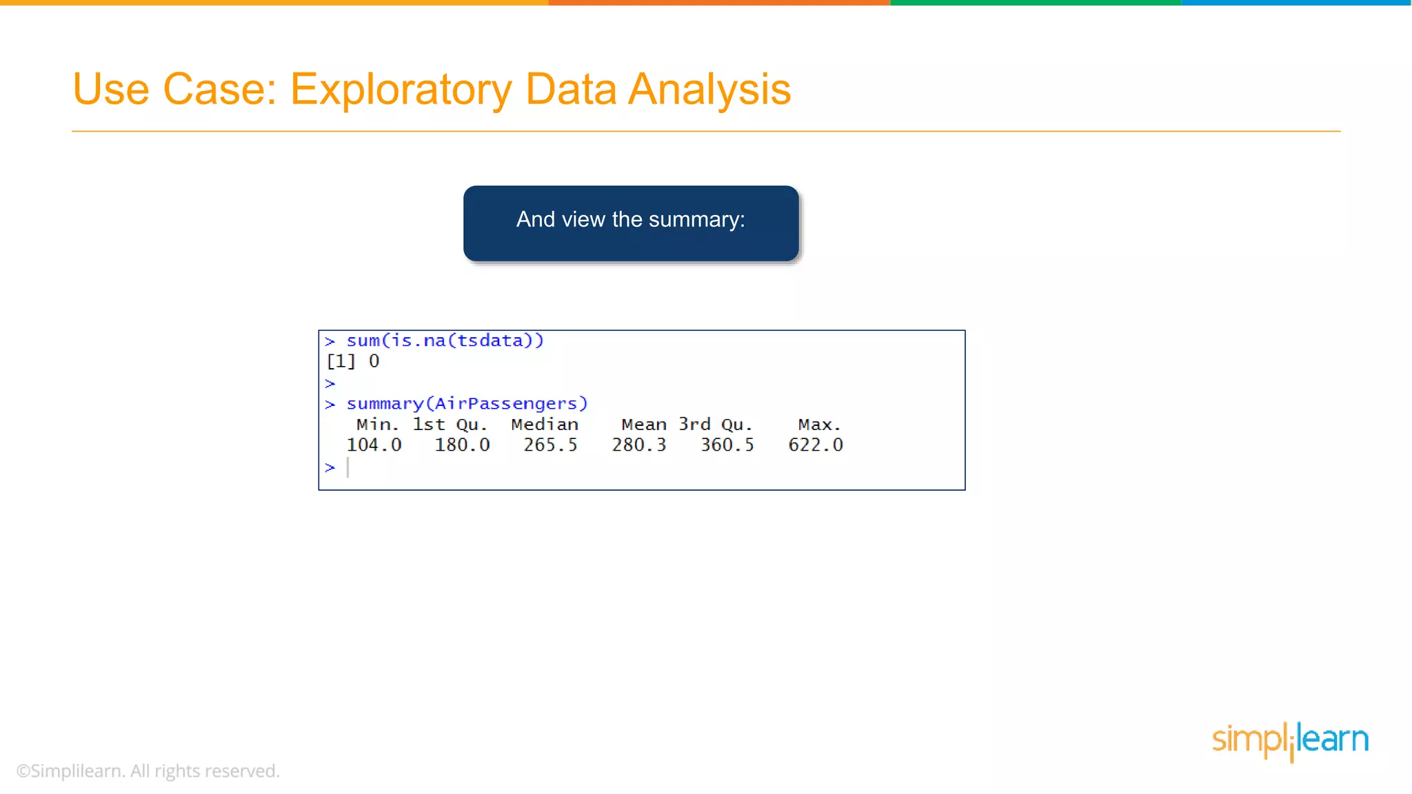
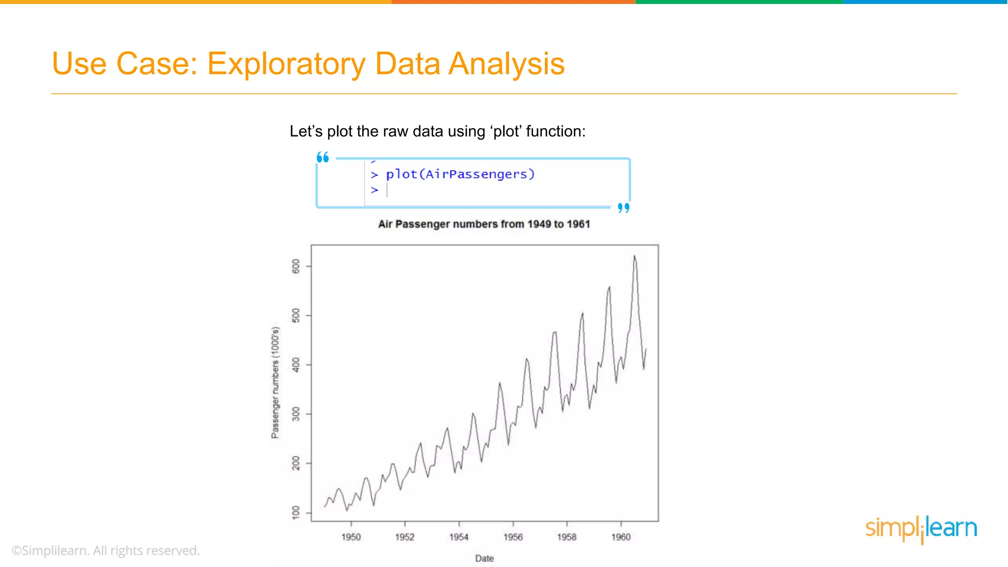
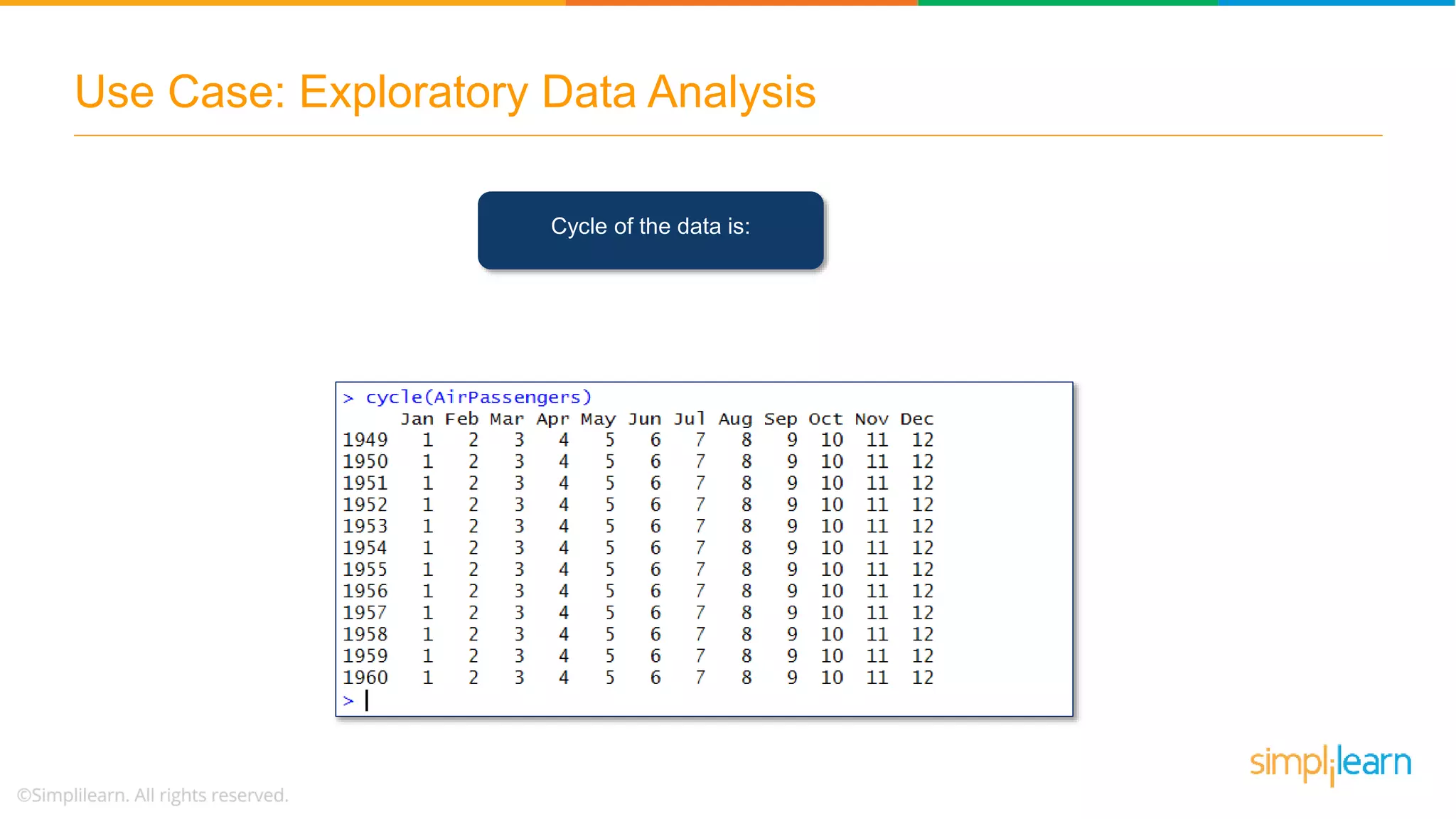
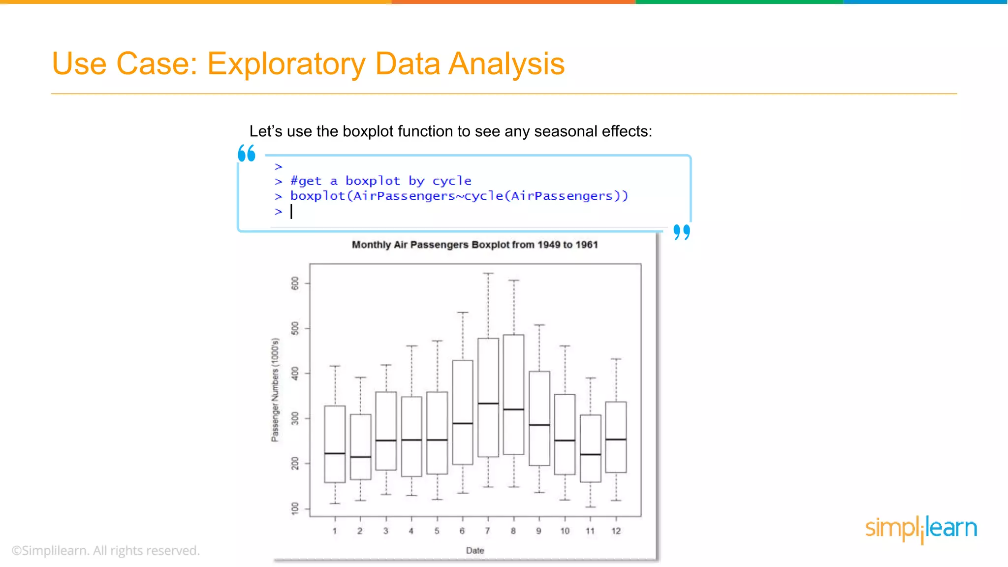
Steps in EDA on Time Series data including loading, checking for missing values, and identifying seasonality and trends.
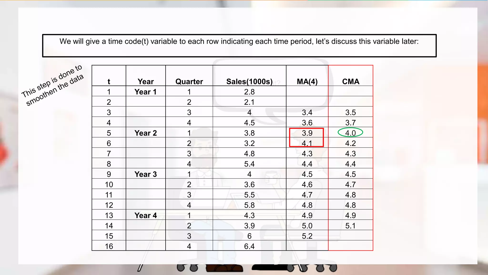
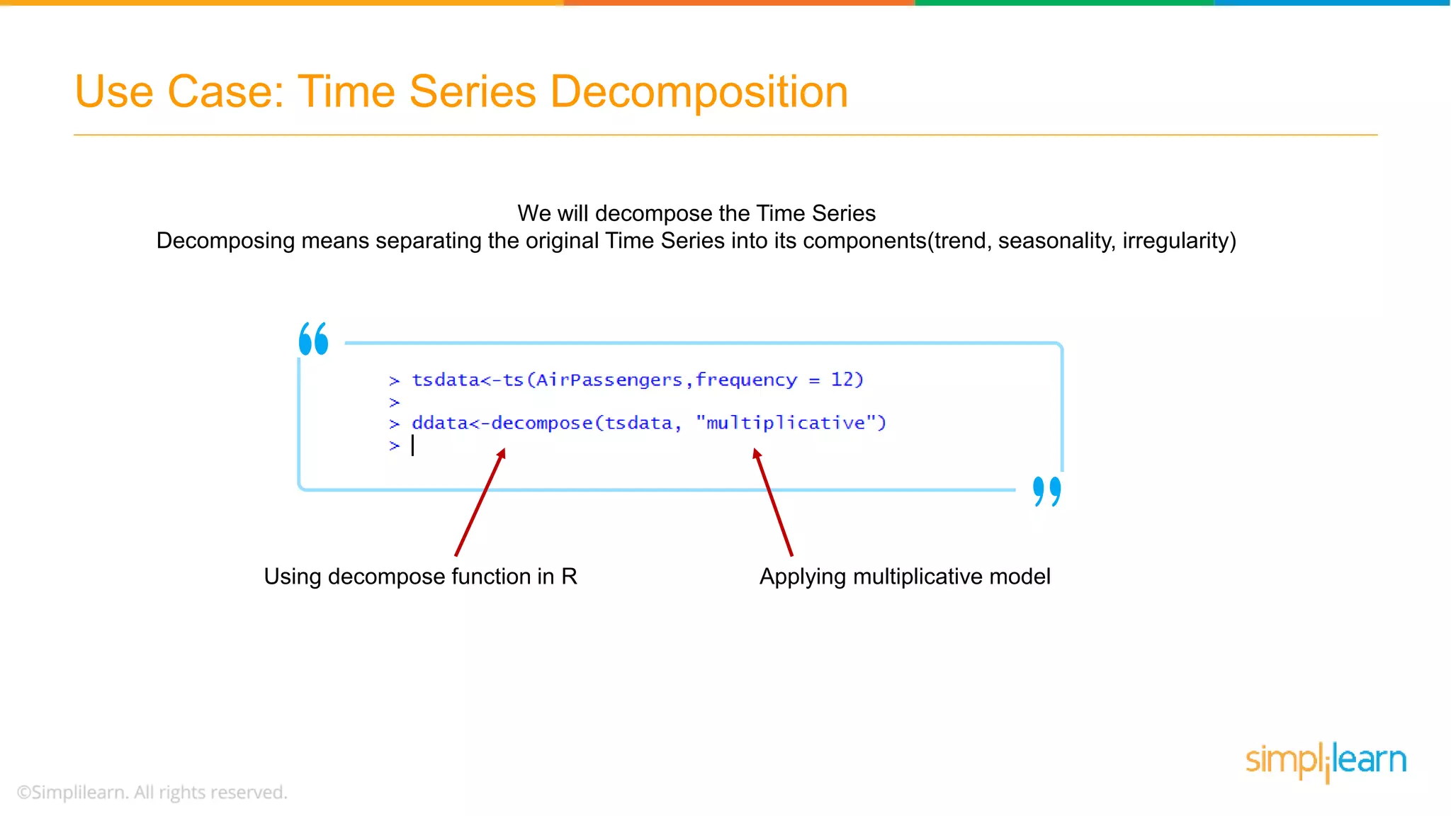
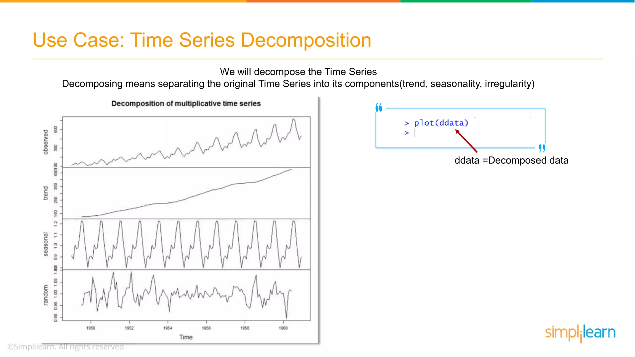
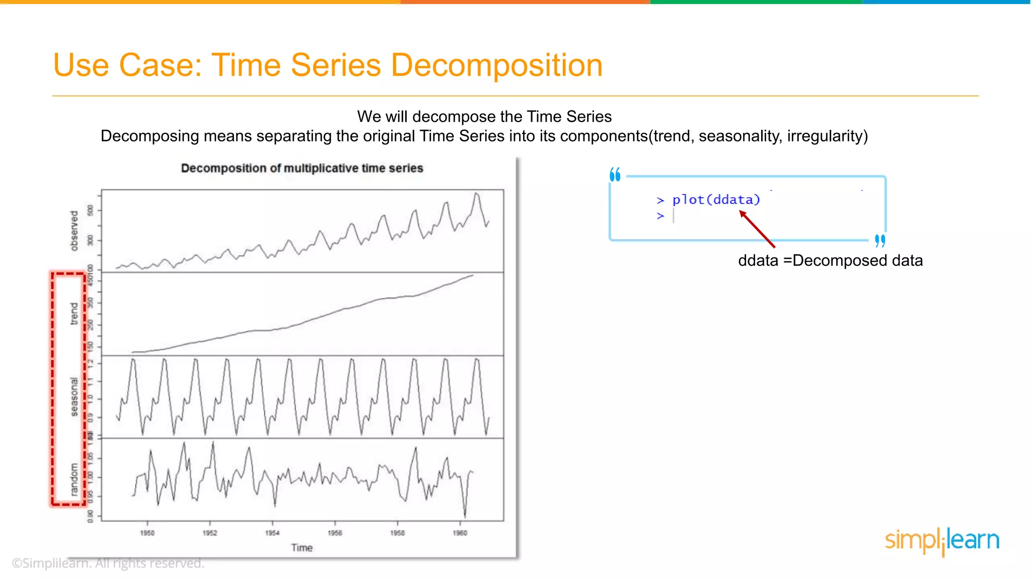
Process of decomposing Time Series data into components—trend, seasonality, and irregularity for analysis.
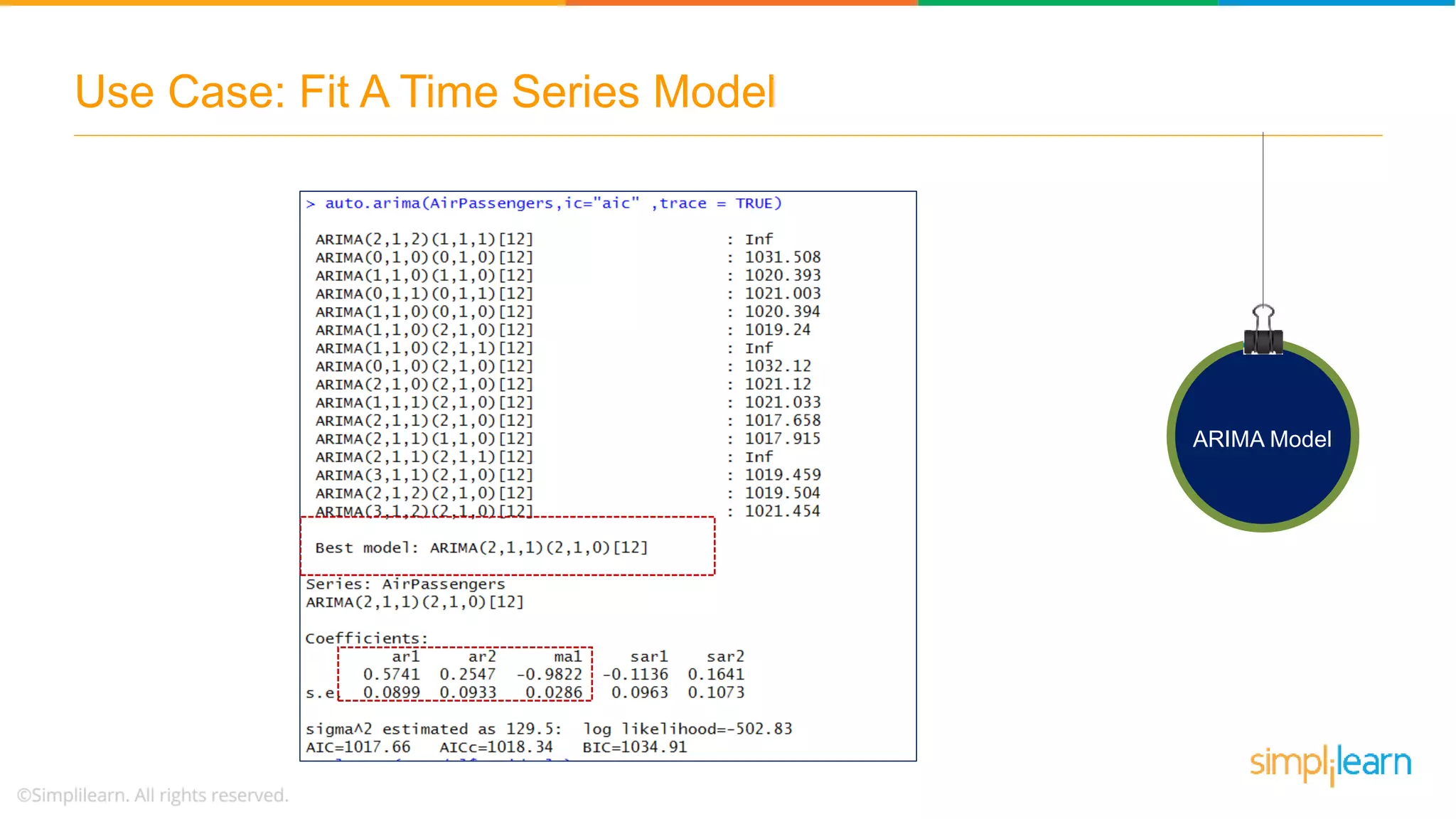
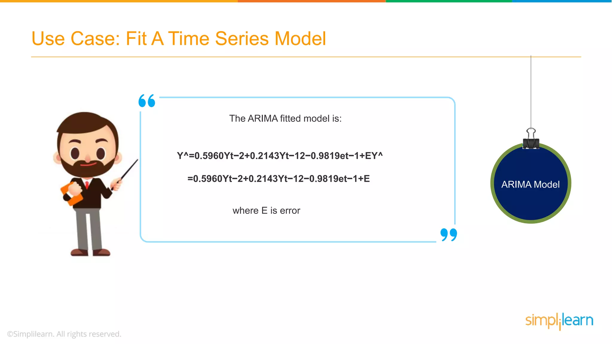
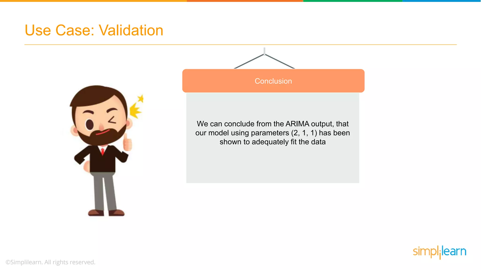
Fitting an ARIMA model to data, highlighting parameters and results of the fitting process.
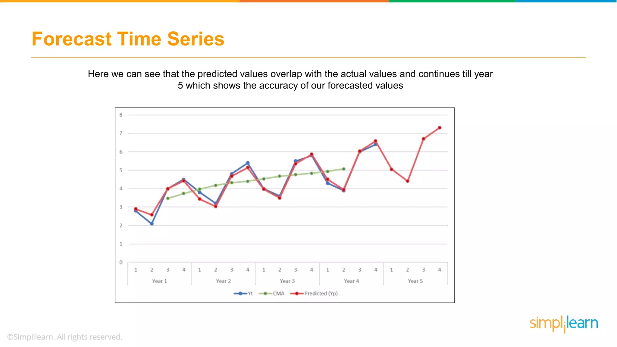
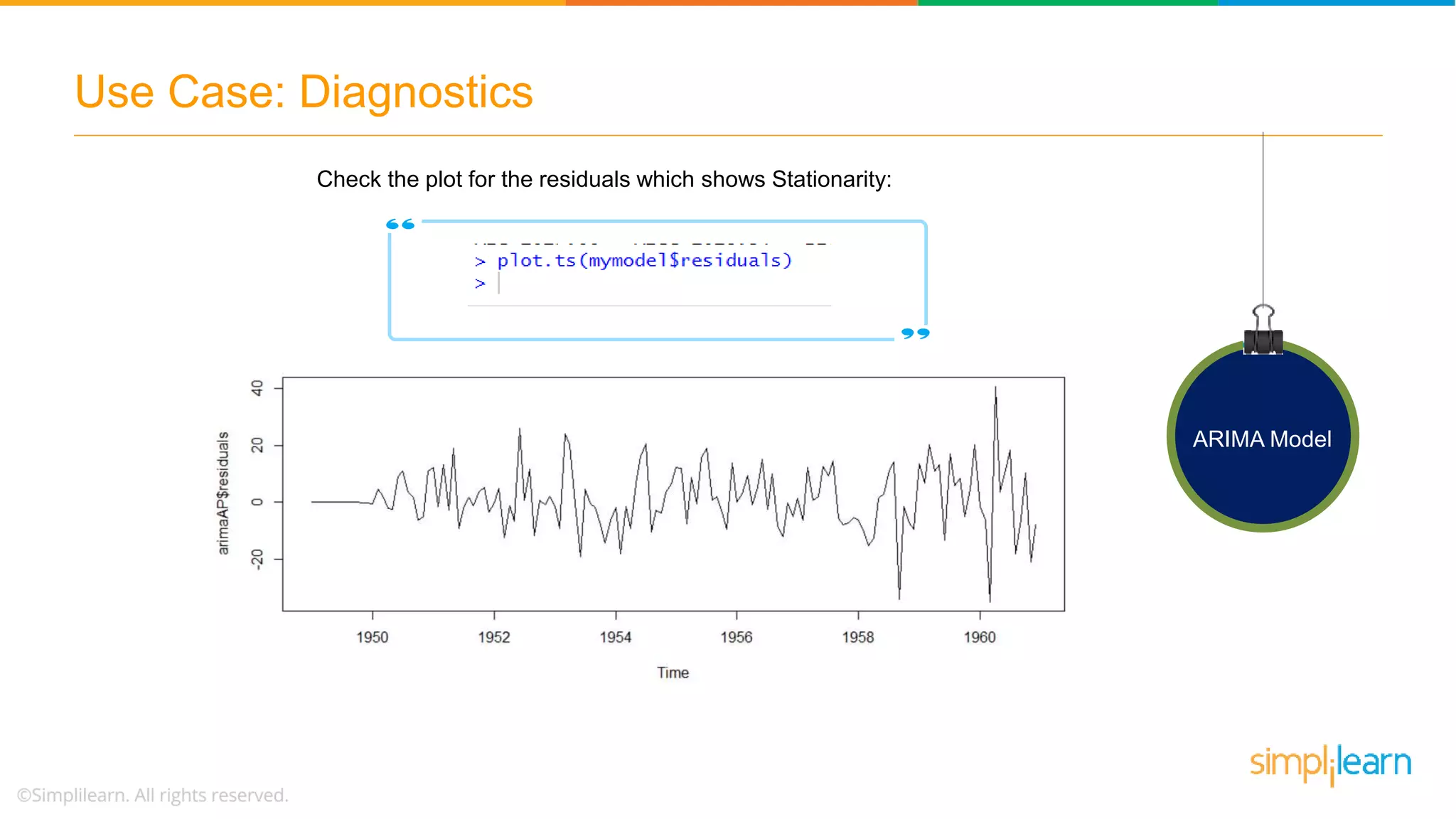
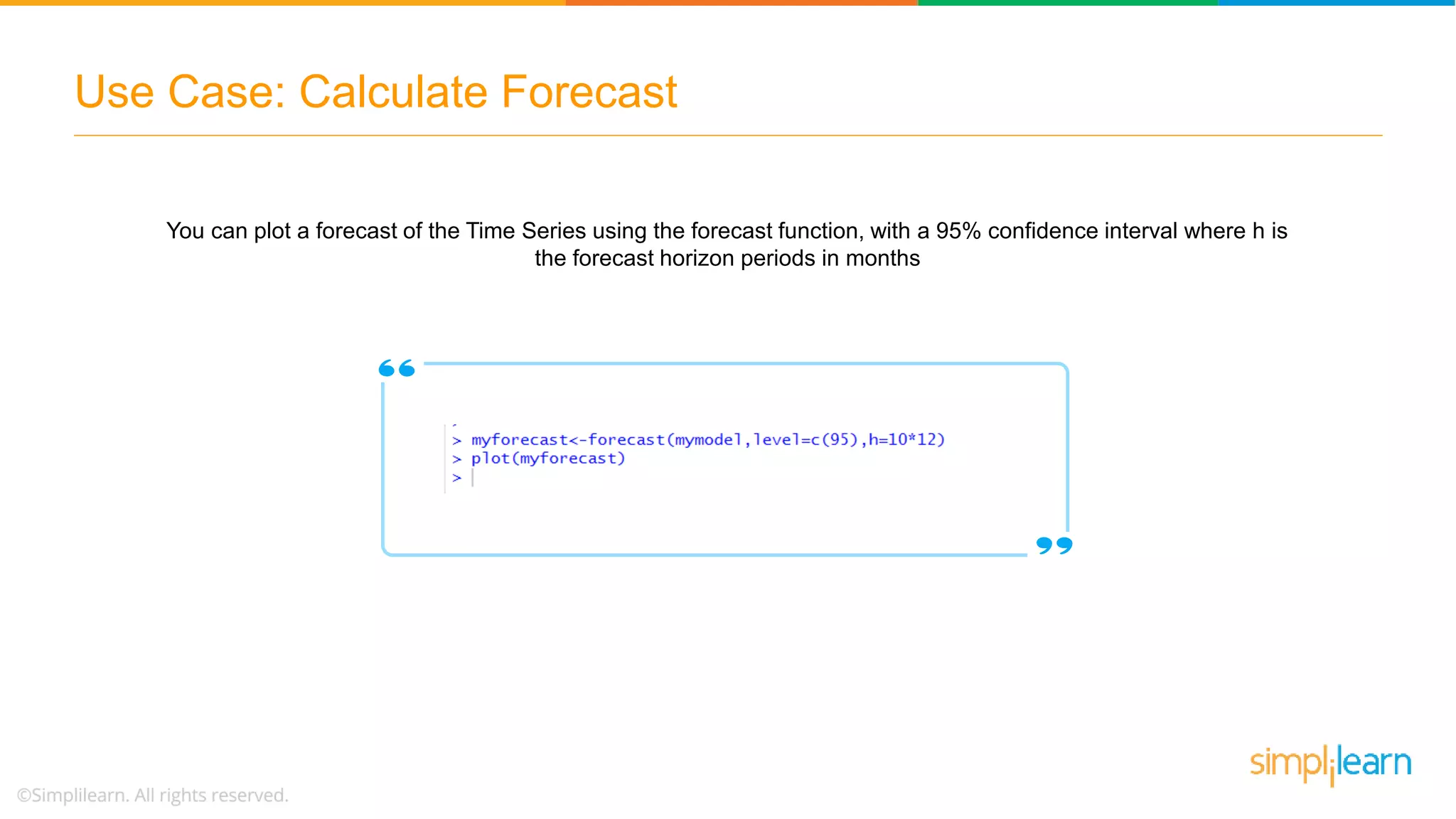
Methods for diagnosing the fit of the ARIMA model including plotting residuals and forecasting.
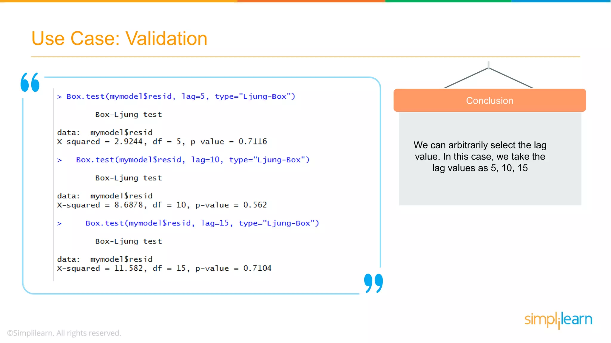
Validation methods for the ARIMA model, specifically using the Ljung-Box test to confirm model accuracy.
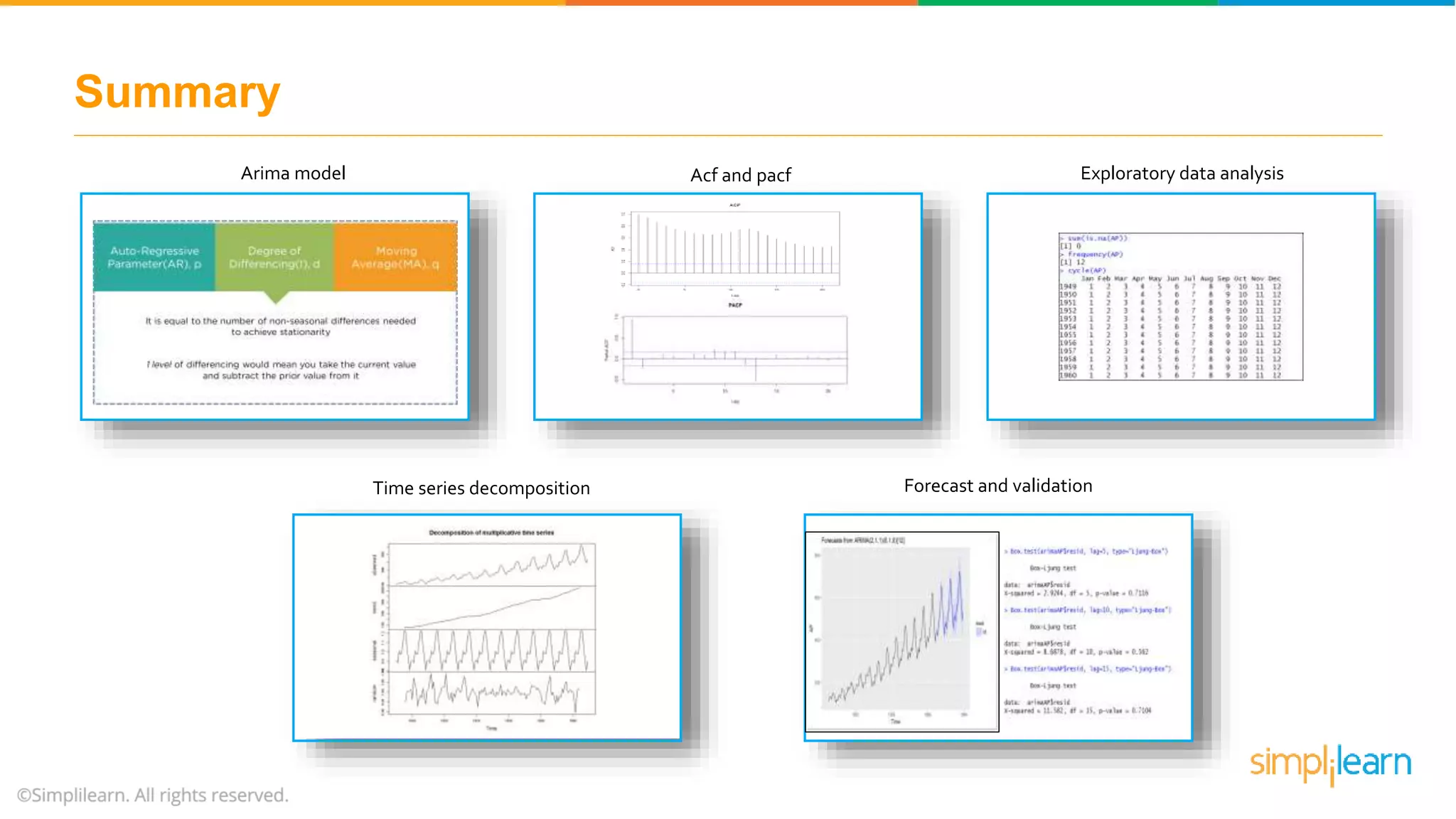
Summary of the critical points covered including ARIMA model, ACF, PACF, exploratory analysis, and forecast validation.


![ARIMA Models - [Lab 3]](https://cdn.slidesharecdn.com/ss_thumbnails/ydqcxn5vtqizjoun2as1-signature-e1de5ad681d661531c2467ca0d3e475440809ccfdbcb78c5369a1bb749945888-poli-141230090527-conversion-gate01-thumbnail.jpg?width=640&height=640&fit=bounds)