AUTO
REGRESSION
Vikas, Sanjay & Aditya
Econometrics MOR204
Auto Regression in Time Series Analysis
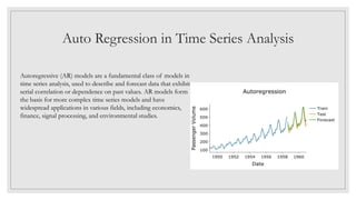
Autoregressive (AR) models are a fundamental class of models in
time series analysis, used to describe and forecast data that exhibit
serial correlation or dependence on past values. AR models form
the basis for more complex time series models and have
widespread applications in various fields, including economics,
finance, signal processing, and environmental studies.
Key Features of an AR Model
• AR models are used to analyze and forecast time series data by exploiting the
relationship between the current value and its past values.
• They are widely used for modeling and forecasting stationary time series data.
• AR models are a crucial component of more advanced models like ARMA and
ARIMA.
• Understanding AR models is essential for time series analysis and forecasting.
Importance of Autoregressive Models in Time
Series Analysis
o Fundamental Building Blocks:
•AR models are the fundamental building blocks for more complex time series
models, such as ARMA (Autoregressive Moving Average) and ARIMA
(Autoregressive Integrated Moving Average) models.
•Understanding AR models is crucial for comprehending and applying these advanced
models effectively.
Importance of Autoregressive Models in Time
Series Analysis
o Modeling Autocorrelation:
• Time series data often exhibit autocorrelation, meaning that the current value is
influenced by its past values.
• AR models are designed to capture and model this autocorrelation structure,
enabling accurate representation and forecasting of time series data.
Importance of Autoregressive Models in Time
Series Analysis
o Stationarity Assumption:
• AR models are particularly useful for analyzing and forecasting stationary time
series, where the statistical properties (mean, variance, and autocorrelation) remain
constant over time.
• Stationarity is a common assumption in many time series applications, making AR
models widely applicable.
Importance of Autoregressive Models in Time
Series Analysis
o Versatile Applications:
• AR models have diverse applications across various domains, including finance
(stock prices, exchange rates), economics (macroeconomic indicators),
environmental studies (air pollution levels, climate patterns), signal processing
(speech recognition, image processing), and more.
• Their versatility stems from their ability to capture and exploit the inherent
autocorrelation structure present in many real-world time series data.
Importance of Autoregressive Models in Time
Series Analysis
o Forecasting Accuracy:
• By accurately modeling the autocorrelation structure, AR models can provide
reliable forecasts, enabling better decision-making and planning in various contexts,
such as inventory management, resource allocation, and risk assessment.
Basics of Autoregression
The current value of the time series is expressed as a finite linear combination of its past values,
plus an error term.
An autoregressive (AR) model is a type of linear regression model where the dependent variable is
regressed on its own lagged values.
 Auto Correlation (AC):
It is a Correlation between the series and past values at certain lag. For instance, lag1 auto
correlation mean correlation between Yt and Yt-1. The idea behind auto correlation is to capture
the serial correlation in the series and use it to improve forecast. Two important uses of AC
AC of original series can help to detect seasonal patterns.
AC of residual series can help to identify remaining information.
Basics of Autoregression
How AC is used by an AR model:
The basic idea behind AR model is to capture AC in a series into a regression type model and use it
to improve short term forecasts. As said before correlation means relationship between variables.
If both variables change in same direction, this is called positive correlation.
If the variables move in opposite direction as value changes then this is called negative correlation.
The stronger the correlation between the output variable and a specific lagged variable, the more
weight that auto regression model can put on that variable when modelling. We can choose which
lag variables will be useful in the model.
Basics of Autoregression
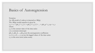
Notation:
An AR model of order p is denoted as AR(p).
The AR(p) model equation is given by
y_t = c + phi_1 * y_t-1 + phi_2 * y_t-2 + ... + phi_p * y_t-p + e_t
where:
y_t is the current value of the time series
c is a constant (intercept)
phi_1, phi_2, ..., phi_p are the autoregressive coefficients
y_t-1, y_t-2, ..., y_t-p are the lagged values of the time series
e_t is the error term (white noise)
Basics of Autoregression
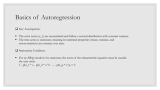
 Key Assumptions:
 The error terms (e_t) are uncorrelated and follow a normal distribution with constant variance.
 The time series is stationary, meaning its statistical properties (mean, variance, and
autocorrelation) are constant over time.
 Stationarity Condition:
 For an AR(p) model to be stationary, the roots of the characteristic equation must lie outside
the unit circle:
1 - phi_1 * z - phi_2 * z^2 - ... - phi_p * z^p = 0
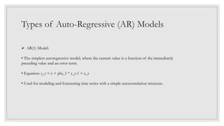
Types of Auto-Regressive (AR) Models
 AR(1) Model:
• The simplest autoregressive model, where the current value is a function of the immediately
preceding value and an error term.
• Equation: y_t = c + phi_1 * y_t-1 + e_t
• Used for modeling and forecasting time series with a simple autocorrelation structure.
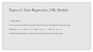
Types of Auto-Regressive (AR) Models
 AR(p) Model:
• A more general autoregressive model, where the current value depends on p previous lags.
• Equation: y_t = c + phi_1 * y_t-1 + phi_2 * y_t-2 + ... + phi_p * y_t-p + e_t
• Useful for capturing more complex autocorrelation patterns in time series data.
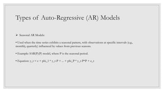
Types of Auto-Regressive (AR) Models
 Seasonal AR Models:
• Used when the time series exhibits a seasonal pattern, with observations at specific intervals (e.g.,
monthly, quarterly) influenced by values from previous seasons.
• Example: SAR(P)(P) model, where P is the seasonal period.
• Equation: y_t = c + phi_1 * y_t-P + ... + phi_P * y_t-P*P + e_t
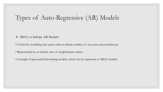
Types of Auto-Regressive (AR) Models
 AR(∞) or Infinite AR Models:
• Useful for modeling time series with an infinite number of non-zero autocorrelations.
• Represented by an infinite sum of weighted past values.
• Example: Exponential Smoothing models, which can be expressed as AR(∞) models.
Types of Auto-Regressive (AR) Models
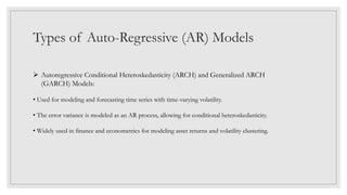
 Autoregressive Conditional Heteroskedasticity (ARCH) and Generalized ARCH
(GARCH) Models:
• Used for modeling and forecasting time series with time-varying volatility.
• The error variance is modeled as an AR process, allowing for conditional heteroskedasticity.
• Widely used in finance and econometrics for modeling asset returns and volatility clustering.
Estimation and Fitting of AR Models
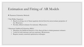
 Parameter Estimation Methods:
• Yule-Walker Equations:
• Based on solving a set of linear equations derived from the autocovariance properties of
the AR process.
• Provides efficient estimates for stationary AR processes.
• Maximum Likelihood Estimation (MLE):
• Maximizes the likelihood function of the observed data to obtain parameter estimates.
• Useful for both stationary and non-stationary AR processes.
• Requires iterative numerical optimization techniques.
Estimation and Fitting of AR Models
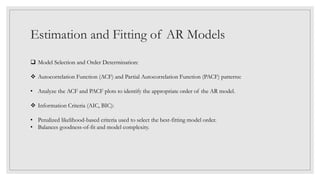
 Model Selection and Order Determination:
 Autocorrelation Function (ACF) and Partial Autocorrelation Function (PACF) patterns:
• Analyze the ACF and PACF plots to identify the appropriate order of the AR model.
 Information Criteria (AIC, BIC):
• Penalized likelihood-based criteria used to select the best-fitting model order.
• Balances goodness-of-fit and model complexity.
Estimation and Fitting of AR Models
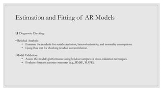
 Diagnostic Checking:
• Residual Analysis:
• Examine the residuals for serial correlation, heteroskedasticity, and normality assumptions.
• Ljung-Box test for checking residual autocorrelation.

•Model Validation:
• Assess the model's performance using holdout samples or cross-validation techniques.

• Evaluate forecast accuracy measures (e.g., RMSE, MAPE).
Estimation and Fitting of AR Models
 Software Implementation:
• Popular software packages for AR model estimation and fitting:
• R: arima() function in the "stats" package, ar() function in the "forecast" package.
• Python: ARIMA class in the "statsmodels" package, AutoReg class in the "pmdarima"
package.
• MATLAB: armax() function, arima() function in the Econometrics Toolbox.
AR Model Implementation
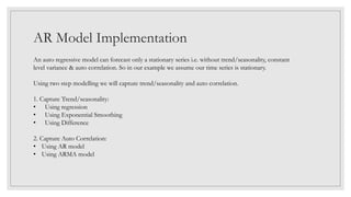
An auto regressive model can forecast only a stationary series i.e. without trend/seasonality, constant
level variance & auto correlation. So in our example we assume our time series is stationary.
Using two step modelling we will capture trend/seasonality and auto correlation.
1. Capture Trend/seasonality:
• Using regression
• Using Exponential Smoothing
• Using Difference
2. Capture Auto Correlation:
• Using AR model
• Using ARMA model
AR Model Implementation
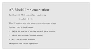
We will start with AR (1) process where 1 stands for lag
Yt=ϕ Yt-1 + C +Εt
Where Et is random white noise with zero mean and constant variance
There are 3 cases we should consider
1. |ϕ|=1, this is the case of unit root, and needs special treatment.
2. |ϕ|<1, series becomes ‘Covariance Stationary’
3. |ϕ|> 1 the process has no bounds.
Among all the cases, case 3 is unpredictable.
AR Model Implementation – An Example
We will go step by step with an example of daily minimum temperatures data set in the city of
Denver over a span of 10 years (1981-1990).
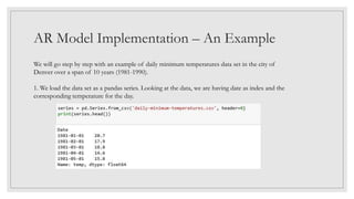
1. We load the data set as a pandas series. Looking at the data, we are having date as index and the
corresponding temperature for the day.
AR Model Implementation – An Example
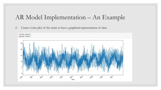
2. Create a Line plot of the series to have a graphical representation of data.
AR Model Implementation – An Example
3. Check for Auto Correlation:
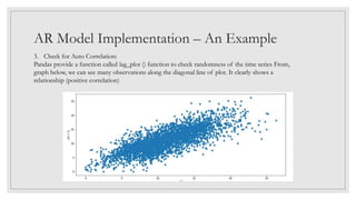
Pandas provide a function called lag_plot () function to check randomness of the time series From,
graph below, we can see many observations along the diagonal line of plot. It clearly shows a
relationship (positive correlation)
AR Model Implementation – An Example
4. Auto Correlation Plots:
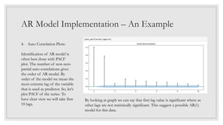
Identification of AR model is
often best done with PACF
plot. The number of non-zero
partial auto correlations gives
the order of AR model. By
order of the model we mean the
most extreme lag of the variable
that is used as predictor. So, let’s
plot PACF of the series. To
have clear view we will take first
10 lags.
By looking at graph we can say that first lag value is significant where as
other lags are not statistically significant. This suggest a possible AR(1)
model for this data.
AR Model Implementation – An Example
5. Persistence Model
Let us consider we are developing a model to forecast last 10 days of minimum temperature. The simplest model
that we could make predictions would be to persist the last observation, we call this as persistence model and can
make use to compare with our auto regression model.
We will split our dataset into training and testing sets, with only last 10 observations in test set that are set as
unseen that we wish to predict.
First, we will create lagged versions of the variable. Before that let’s see the use of lagged versions of the variable
in regression model.
• This allows varying amounts of recent history to be brought into forecast.
• Lagging of independent variables is often necessary for the regression model to be able to predict the future--
i.e., to predict what will happen in period t based on knowledge of what happened up to period t-1.
AR Model Implementation – An Example
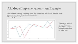
Now divide the series into training and testing data sets and using walk-forward validation we can
persist the most recent observations for the next day.
The sample plot looks like:
The expected values for
the next 10 days are
plotted (blue) compared
to the predictions from
the model (red).
AR Model Implementation – An Example
6. AR Model
In an AR model, we use lagged variables as input variables. The statsmodels library provides an auto
regression model that automatically selects an appropriate lag value using statistical tests and trains a
linear regression model. It is provided in the AR class.
We will first create a model AR () and then calling ‘fit ()’ to train it on our dataset. With resultant AR
Result object, we can predict by calling predict () function for many observations in future. This
creates 1 10-day forecast (assuming we are creating forecast for 10 days).
Split the dataset into train data and test data, as we are doing forecast for 10 days we will make test
data with only last 10 observations of dataset as unseen data that we wish to predict.
Now make predictions and calculate mean-square error.
AR Model Implementation – An Example
Plot Predictions:
When you plot the graph, most of the predictions are close but there might be deviations too.
One way would be re-train the AR model each day with new observations. We can make use of
another alternative which is to use the learned coefficients and use them manually to make
predictions.
The coefficients are provided in an array with the intercept term followed by the coefficients for each
lag variable starting at t-1 to t-n. We simply need to use them in the right order.
AR Model Implementation – An Example
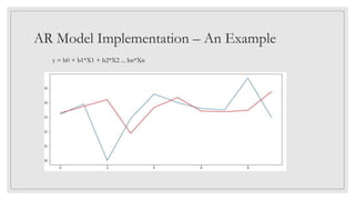
y = b0 + b1*X1 + b2*X2 ... bn*Xn
Importance of an AR Model
• The Autoregression Model holds significant importance in time series analysis and forecasting
due to several key reasons. It allows analysts to capture and model the inherent dynamics and
patterns present in sequential data, enabling them to understand the relationships between past
and future observations.
• Additionally, autoregressive models serve as a foundation for more advanced time series models
like ARIMA and SARIMA, offering a framework for analyzing and modeling complex temporal
data.
• By understanding and implementing autoregression techniques, analysts can improve the
accuracy of their forecasts, identify anomalies or trends in the data, and make informed
predictions for future outcomes.
• Overall, the Autoregression Model is essential for extracting meaningful insights from time series
data and enhancing predictive capabilities in various domains.
Applications of Auto Regressive Models
 Finance and Economics:
• Forecasting stock prices, exchange rates, and economic indicators (e.g., GDP, inflation,
unemployment rates).
• Modeling and predicting volatility in financial markets using GARCH models.
• Analyzing and forecasting interest rates and yield curves.
 Environmental Studies:
• Modeling and forecasting air pollution levels, water quality, and climate patterns.
• Predicting future values of environmental variables based on historical data.
• Assessing the impact of policy changes or interventions on environmental indicators.
Applications of Auto Regressive Models
 Signal Processing:
• Speech recognition and synthesis.
• Image processing and compression.
• Modeling and forecasting time-varying signals in various applications.
 Healthcare and Biomedical:
• Modeling and forecasting disease incidence rates and epidemiological trends.
• Analyzing and predicting patient health outcomes and treatment responses.
• Modeling and forecasting biomedical signals (e.g., ECG, EEG).
 Transportation and Logistics:
• Forecasting traffic patterns and optimizing transportation routes.
• Modeling and predicting demand for transportation services.
• Optimizing resource allocation and scheduling in logistics operations.
Limitations and Challenges in AR Modeling
 Stationarity Assumption:
• AR models assume that the time series is stationary, meaning its statistical properties (mean, variance, and
autocorrelation) remain constant over time.
• Non-stationary time series may require differencing or other transformations to achieve stationarity, which
can lead to complexity and potential information loss.
 Model Order Selection:
• Determining the appropriate order (p) of the AR model is crucial but can be challenging, especially for
complex time series with multiple autocorrelation patterns.
• Underspecifying or overspecifying the model order can lead to biased parameter estimates and poor
forecasting performance.
 Outliers and Structural Breaks:
• AR models can be sensitive to outliers and structural breaks (sudden shifts) in the time series data.
• Outliers and breaks can distort the autocorrelation structure, leading to biased parameter estimates and
inaccurate forecasts.
Bibliography
 Books
 Wikipedia
 LinkedIn
 General Articles
 machinelearningmastery.com
Thank You!