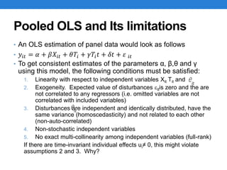
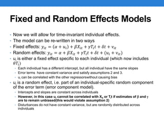
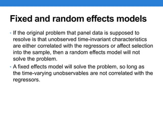
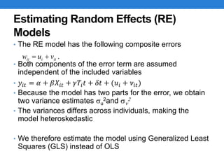
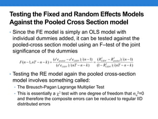
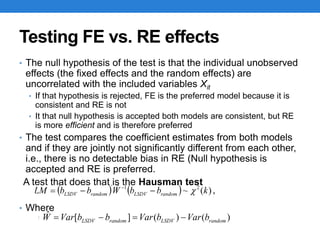
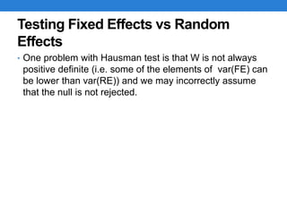
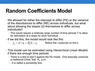
The document focuses on the use of panel data models for econometric analysis, specifically detailing pooled OLS and its limitations, as well as fixed and random effects models. It describes the necessary conditions for consistent parameter estimation and how unobserved time-invariant characteristics can be accounted for using these models. Additionally, it discusses methods for estimating and testing the validity of fixed and random effects models against pooled cross-section models, including the Hausman test.

1. Panel Data Models
Day 2, Lecture 2
By Ragui Assaad
Training on Applied Micro-Econometrics and
Public Policy Evaluation
July 25-27, 2016
Economic Research Forum

2. Pooled OLS and Its limitations
• An OLS estimation of panel data would look as follows
• 𝑦𝑖𝑡 = 𝛼 + 𝛽𝑋𝑖𝑡 + 𝜃𝑇𝑖 + 𝛾𝑇𝑖 𝑡 + 𝛿𝑡 + 𝜀 𝑖𝑡
• To get consistent estimates of the parameters α, β,θ and γ
using this model, the following conditions must be satisfied:
1. Linearity with respect to independent variables Xit Tit and
2. Exogeneity. Expected value of disturbances eitis zero and the are
not correlated to any regressors (i.e. omitted variables are not
correlated with included variables)
3. Disturbances are independent and identically distributed, have the
same variance (homoscedasticity) and not related to each other
(non-auto-correlated)
4. Non-stochastic independent variables
5. No exact multi-collinearity among independent variables (full-rank)
If there are time-invariant individual effects ui≠ 0, this might violate
assumptions 2 and 3. Why?
eit
eit

3. Fixed and Random Effects Models
• Now we will allow for time-invariant individual effects.
• The model can be re-written in two ways
• Fixed effects: 𝑦𝑖𝑡 = 𝛼 + 𝑢𝑖 + 𝛽𝑋𝑖𝑡 + 𝛾𝑇𝑖 𝑡 + 𝛿𝑡 + 𝜈𝑖𝑡
• Random effects: 𝑦𝑖𝑡 = 𝛼 + 𝛽𝑋𝑖𝑡 + 𝛾𝑇𝑖 𝑡 + 𝛿𝑡 + (𝑢𝑖 + 𝜈𝑖𝑡)
• ui is either a fixed effect specific to each individual (which now includes
𝜃𝑇𝑖)
• Each individual has a different intercept, but all individual have the same slopes
• Error terms have constant variance and satisfy assumptions 2 and 3.
• ui can be correlated with the other regressorswithout causing bias
• ui is a random effect, i.e. part of an individual-specific random component
of the error term (error component model).
• Intercepts and slopes are constant across individuals
• However, in this case ui cannot be correlated with Xit or Tit if estimates of b and g
are to remain unbiased(this would violate assumption 2)
• Disturbances do not have constant variance, but are randomly distributed across
individuals

4. Fixed and random effects models
• If the original problem that panel data is supposed to
resolve is that unobserved time-invariant characteristics
are either correlated with the regressors or affect selection
into the sample, then a random effects model will not
solve the problem.
• A fixed effects model will solve the problem, so long as
the time-varying unobservables are not correlated with the
regressors.

5. Estimating Fixed Effects (FE) Model
• Fixed effect models can be estimated using the Least
Squares Dummy Variable Model (LSDV)
• This consists of including a dummy variable for each individual in
the data except for one (the reference)
• If the number of individuals is large and the number of period is
small we do not get consistent estimates of the fixed effects
themselves, but the other coefficients of the model are consistently
estimated.
• Alternative is the “within estimation” model
• Consists of taking differences across individuals and estimating
using these first differences
• “Within estimator” model produces wrong standard errors that must be
corrected

6. Estimating Random Effects (RE)
Models
• The RE model has the following composite errors
• Both components of the error term are assumed
independent of the included variables
• 𝑦𝑖𝑡 = 𝛼 + 𝛽𝑋𝑖𝑡 + 𝛾𝑇𝑖 𝑡 + 𝛿𝑡 + (𝑢𝑖 + 𝜈𝑖𝑡)
• Because the model has two parts for the error, we obtain
two variance estimates su
2and sn
2
• The variances differs across individuals, making the
model heteroskedastic
• We therefore estimate the model using Generalized Least
Squares (GLS) instead of OLS

7. Testing the Fixed and Random Effects Models
Against the Pooled Cross Section model
• Since the FE model is simply an OLS model with
individual dummies added, it can be tested against the
pooled-cross section model using an F–test of the joint
significance of the dummies
• Testing the RE model again the pooled cross-section
model involves something called:
• The Breusch-Pagan Lagrange Multiplier Test
• This is essentially a c2 test with one degree of freedom that su
2=0
and therefore the composite errors can be reduced to regular IID
distributed errors

8. Testing FE vs. RE effects
• The null hypothesis of the test is that the individual unobserved
effects (the fixed effects and the random effects) are
uncorrelated with the included variables Xit
• If that hypothesis is rejected, FE is the preferred model because it is
consistent and RE is not
• It that null hypothesis is accepted both models are consistent, but RE
is more efficient and is therefore preferred
• The test compares the coefficient estimates from both models
and if they are jointly not significantly different from each other,
i.e., there is no detectable bias in RE (Null hypothesis is
accepted and RE is preferred.
A test that does that is the Hausman test
• Where

9. Testing Fixed Effects vs Random
Effects
• One problem with Hausman test is that W is not always
positive definite (i.e. some of the elements of var(FE) can
be lower than var(RE)) and we may incorrectly assume
that the null is not rejected.

10. Random Coefficients Model
• We allowed for either the intercept to differ (FE) or the variance
of the disturbances to differ (RE) across individuals, but what
about allowing the slopes (b) themselves to differ across
individuals?
• This would require a relatively large number of time periods T to allow
for estimation of a slope for each individual
• If we did this, the model would look like this
• Notice the i subscript on the b
• This model can be estimated using Hierarchical Linear Models
if there are enough time periods.
• There is a test to test it against the FE model. One basically conducts
a traditional Chow Test H0: bi=b
• . It is called a poolability test.
yit =a +ui + ¢Xitbi +vit