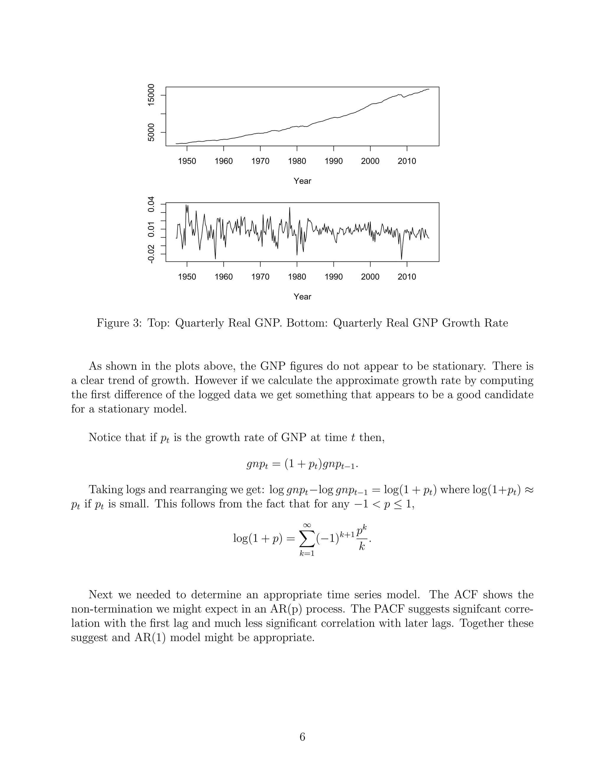
This document discusses using bootstrap methods to create confidence intervals for time series forecasts. It provides examples of time series data and introduces the AR(1) model. The document describes an algorithm for calculating a bootstrap confidence interval for forecasting from an AR(1) model. It then discusses a simulation study comparing empirical coverage rates of bootstrap confidence intervals under different parameters. Finally, it applies the bootstrap method to forecasting Gross National Product growth, comparing the results to a parametric approach.

1. Timeseries and Bootstrap-Based Confidence Intervals
for Forecasting
Chelsey Erway, Karl Rudeen, Brian Whetter
June 9, 2016

2. 1 Introduction
In this report we will discuss some preliminaries about time series in general then explore
how we can apply bootstrap methods to create confidence intervals for forecasts from time
series data. Following Shumway and Stover [3], we first give some examples of times series
data, introduce the AR(1) model and the Partial Autocorrelation Function (PACF). We then
give an algorithm for calculating a bootstrap confidence interval of a forecast as discussed
in Chernick and LaBudde [1]. In the latter parts of the paper we use a modification of
their R code (pp 120-122) to conduct a simulation study and an application with real data.
In Section 5, we discuss the simulation process and report empirical coverage rates for our
bootstrap confidence intervals. In Section 6, we apply an AR(1) model Gross National
Product (GNP) growth data, comparing bootstrap and parametric approaches.
2 Time Series Basics
For our purposes, a time series is a sequence of data points spaced equally over time. In
general, the correlation between two adjacent points make it difficult to apply conventional
statistical methods that rely on the random variables being independent and identically dis-
tributed. However, with an appropriate time series model, one can make reasonably accurate
predictions about future values. First we give some basic examples and introduce some def-
initions.
A simple example of a time series model is a random walk with drift. Let
xt = δ + xt−1 + wt
where δ is some drift constant, and wt is some white noise coming from a distribution with
mean 0. For example, wt ∼ N(0, 1). If δ = 0, the model is simply a random walk. We will
use the above example to help illustrate a few concepts and definitions.
The mean function is defined by
µxt = E(xt)
or, when the time series is clearly specified, simply µt. Since we can write the random walk
with drift as xt = δt + t−1
j=1 wj, we get
µt = E(xt) = δt +
t−1
j=1
E(wj) = δt.
The autovariance funtion is defined by
γx(s, t) = cov(xs, xt) = E[(xs − µs)(xt − µt)].
The autocovariance function measures the linear dependence between two points. For the
random walk model with wt ∼ N(0, σ2
) we get
γx(s, t) = cov(xs, xt) = cov
s
j=1
wj,
t
j=1
wj = min{s, t}σ2
.
1

3. The autocovariance function can be normalized to obtain the autocorrelation function
(ACF) written as
ρ(s, t) =
γ(s, t)
γ(s, s)γ(t, t)
.
The ACF measures the linear predictability between two variables in a time series. Using
the Cauchy-Schwartz inequality we get −1 ≤ ρ(s, t) ≤ 1.
In this paper we restrict our discussion to stationary time series. A time series is weakly
stationary if
(i) the mean value function µt is constant and does not depend on time, and
(ii) the autocovariance function, γ(s, t) depends on s and t only through their difference
|s − t|.
For now on we use the term stationary to mean weakly stationary.
Notice that a random walk and a random walk with drift are both non-stationary. The
random walk with drift fails both conditions (i) and (ii). A random walk passes condition
(i) but fails condition (ii).
For a stationary times series we now have
γ(h) = cov(xt+h, xt) = E[(xt+h − µ)(xt − µ)]
and
ρ(h) =
γ(h)
γ(0)
.
3 Autoregressive Models and The PACF
In what follows we will restrict our attention to the Autoregressive Model of order 1. An
Autoregressive Model of order p or AR(p), is a model of the form
xt = β1xt−1 + β2xt−2 + · · · + βpxp + et
where βi, 1 ≤ i ≤ p are nonzero constants, and the error terms et are iid random variables.
It is convenient to have E[xt] = 0. If E[xt] = 0, we replace xt with xt − E[xt].
We note here a theoretical result: given an AR(p) model, xt = β1xt−1 + · · · + βpxp + et,
we can associate it with the polynomial equation p(x) = xp
− β1xp−1
− · · · − βp−1x − βp with
real coefficients and roots in the complex plane. In order for stationarity to hold, all roots
of the polynomial must fall strictly inside the unit circle of the complex plane. In particular
for AR(1) we have p(x) = x − β, and so stationarity holds if |β| < 1.
A natural question is how to determine the appropriate value of p for a given time se-
ries. Prima facie, one might think that the ACF would be sufficient way to determine p. It
2

4. Figure 1: The ACF and the PACF of an AR(2) model with β1 = 1.5 and β2 = −.75
turns out, however, that the ACF for an AR(p) model does not level out for any lag, and
consequently it is very difficult to determine a good cut point between the significant and
insignificant lags. Fortunately, there is an alternative diagnostic tool.
We define the partial autocorrelation function (PACF) of xt, denoted by φhh, for
h = 1, 2, . . . , as
φ11 = cor(x1, x0) = ρ(1)
and
φhh = cor(xh − xh, x0 − x0), h ≥ 2,
where xh is the regression of xh on {x1, x2, . . . xh−1} and x0 is the regression of x0 on
{x1, x2, . . . xh−1}.
The problem with the ACF is that one variable, say xs, can be correlated with another
variable xt via another member in the series between them, say xr where t < r < s. The
PACF measures the correlation between xs and xt with the linear effect of “everything in
the middle” removed. The merit of the PACF in contrast to the ACF for AR(p) models is
demonstrated in Figure 1 where it is easy to see from the PACF that the first two lags are
significant, suggesting the data is AR(2).
4 Bootstrap Forecasting for Stationary AR(1) Models
Here we give an algorithm for computing a percentile-based confidence interval for a forecast.
We give a procedure for AR(1) models which could be adapted to AR(p).
1. Given an original time series of length r calculate ˆβ using least squares.
2. Using the ˆβ value, gather a vector of residuals calculated by ˆet = xt − ˆβxt−1
3

5. 3. Resample B times from ˆe = {ˆe1, . . . ˆer} using either bootstrap or permutation to get
ˆe(b)
= {ˆe
(b)
1 , . . . , ˆe
(b)
r }.
4. Generate a new time series x
(b)
t = x
(b
t−1 +ˆe
(b)
t . For each new time series, use least squares
again to find a new estimate for β, ˆβ(b)
.
5. For each resample, calculate an estimate for ˆxr+1 by ˆx
(b)
r+1 = ˆβ(b)
x
(b)
r .
6. Create a percentile-based confidence interval from the set {ˆx
(1)
r+1, ˆx
(2)
r+1, . . . , ˆx
(B)
r+1}
Notice that since we calculated the set {ˆβ(1)
, ˆβ(2)
, . . . , ˆβ(B)
}, we could also create a per-
centile based confidence interval for β.
If we know our errors have a certain distribution, say et ∼ N(0, 1), then we can use a
parametric process to generate a confidence interval as well. In the last section we compare
the bootstrap and parametric methods in an application to GNP data.
5 A Simulation Study
We created a function, bigfunction, that takes a β value as an input and generates a time
series based on the given value and randomly generated white noise errors. The very last
entry of the time series is removed from the vector and saved in a numeric variable, correct-
forecast. The code then applies the bootstrapping procedure to the remainder of the time
series and creates a 95% confidence interval for the forecast. The function now returns a 1 if
correctforecast falls inside the confidence interval, and a 0 if it does not. From this function
we simply use apply to run the code 1000 times and calculate the empirical coverage rate.
It is worth noting that the part of our function, tsboot that did most of the bootstrap-
ping would throw errors from time to time. This is not an issue when creating a single
confidence interval, but when one wants to run the function 1000 times, the error was sure
to happen at least once, thus ruining the entire process. We dealt with this by including a
tryCatch block, and using if statements to return a −1 if the function failed. It is unclear
what was causing the error. However, it is possible that the resamples that were created
were sometimes not AR(1), which would cause the program to fail.
We completed eleven simulation studies on time series generated using different param-
eters. In particularly, we varied β, the time series length, l, and variance of the white noise
et. For eight of the eleven studies we used a normal distribution with zero mean to generate
white noise. For the remaining three we used uniformly distributed white noise.
Results
The table in Figure 2 shows the parameters used for each simulation and the resulting cov-
erage rates, r. Most fell somewhere between 89% and 93%. Note that the coverage rate was
highest for Trial 6 where the value of β was closest to 1. The follows the general patten that
4

6. Trial Number β l et r
Trial 1 0.7 100 N(0, 1) 90 %
Trial 2 0.7 200 N(0, 1) 93 %
Trial 3 0.7 300 N(0, 1) 92 %
Trial 4 0.4 200 N(0, 1) 65 %
Trial 5* 0.2 200 N(0, 1) NA
Trial 6 0.9 200 N(0, 1) 99 %
Trial 7 0.7 200 N(0, 2) 92 %
Trial 8 0.7 200 N(0, 1
2
) 91 %
Trial 9 0.7 200 Unif(−1, 1) 90 %
Trial 10 0.7 200 Unif(−1
2
, 1
2
) 89 %
Trial 11 0.7 200 Unif(−2, 2) 92 %
Figure 2: Coverage Rates for Different Simulations
coverage rates are higher for larger values of β. It appears that the length of the time series
data had at best a very small impact on the coverage rates. Similarly, the coverage rate
seemed relatively unaffected by changes in the variance of the residuals, or even by changing
the residual distribution to a uniform distribution.
We also noticed the β values seemed to have a large impact on the rate of errors thrown
as discussed above. When β was reduced to .4, we found that the coverage rate decreased
substantially. At the same time, the error rate increased substantially. For β = .2, the
number of errors thrown was nearly 100% so were unable to generate a meaningful coverage
rate.
6 Application: Forecasting GNP
To demonstrate a scenario in which we might want to bootstrap forecasts from an AR(1)
model, we considered Gross National Product (GNP) values, gnp, for the United States be-
tween the first quarter of 1947 and the first quarter of 2016. Specifically, we looked at real,
seasonally-adjusted quarterly data in 2009 dollars. Our goal here is to compute a forecast
for the next period, that is, to answer the question what will GNP be for the second quarter
of 2016?
5

7. Year
1950 1960 1970 1980 1990 2000 2010
500015000
Year
1950 1960 1970 1980 1990 2000 2010
-0.020.010.04
Figure 3: Top: Quarterly Real GNP. Bottom: Quarterly Real GNP Growth Rate
As shown in the plots above, the GNP figures do not appear to be stationary. There is
a clear trend of growth. However if we calculate the approximate growth rate by computing
the first difference of the logged data we get something that appears to be a good candidate
for a stationary model.
Notice that if pt is the growth rate of GNP at time t then,
gnpt = (1 + pt)gnpt−1.
Taking logs and rearranging we get: log gnpt−log gnpt−1 = log(1 + pt) where log(1+pt) ≈
pt if pt is small. This follows from the fact that for any −1 < p ≤ 1,
log(1 + p) =
∞
k=1
(−1)k+1 pk
k
.
Next we needed to determine an appropriate time series model. The ACF shows the
non-termination we might expect in an AR(p) process. The PACF suggests signifcant corre-
lation with the first lag and much less significant correlation with later lags. Together these
suggest and AR(1) model might be appropriate.
6

8. 0 2 4 6 8 10
0.00.40.8
Lag (Quarters)
ACF
2 4 6 8 10
-0.10.10.3
Lag(Quarters)
PACF
Series as.vector(gnpgr)
Figure 4: ACF and PACF for GNP Growth Rate
After transforming our data by letting xt = log gnpt − log gnpt−1, we also center it to
obtain yt = xt − ¯x. Now we want to estimate the AR(1) model:
yt = βyt−1 + et.
6.1 A Parametric Confidence Interval
First we use the ar function in R to estimate the model using OLS. If the process we are
modeling is stationary, and the errors are uncorrelated and normally distributed then we can
expect OLS to give us an unbiased estimate for β. We obtain the following:
ˆβ .367
Var of ˆβ 0.003146
Forecast Growth Rate .004731
Forecast Growth Rate CI (0.003820.00564)
Forecast CI (dollars) (16686.83, 16717.23)
Based on this estimate we expect GNP in 2016 Q2 to be between about $16,687 and
$16,717.
An OLS estimate of β has theoretical variance Var(ˆβ) ≈ 1−ˆβ2
n
≈ 0.003135 which closely
matches the value computed by R. In the next section we will verify this using bootstrap.
One of our assumptions about our model is that the errors, et, are uncorrelated. We can
check this assumption by looking at the PACF of the residuals ˆet in our estimated model.
7

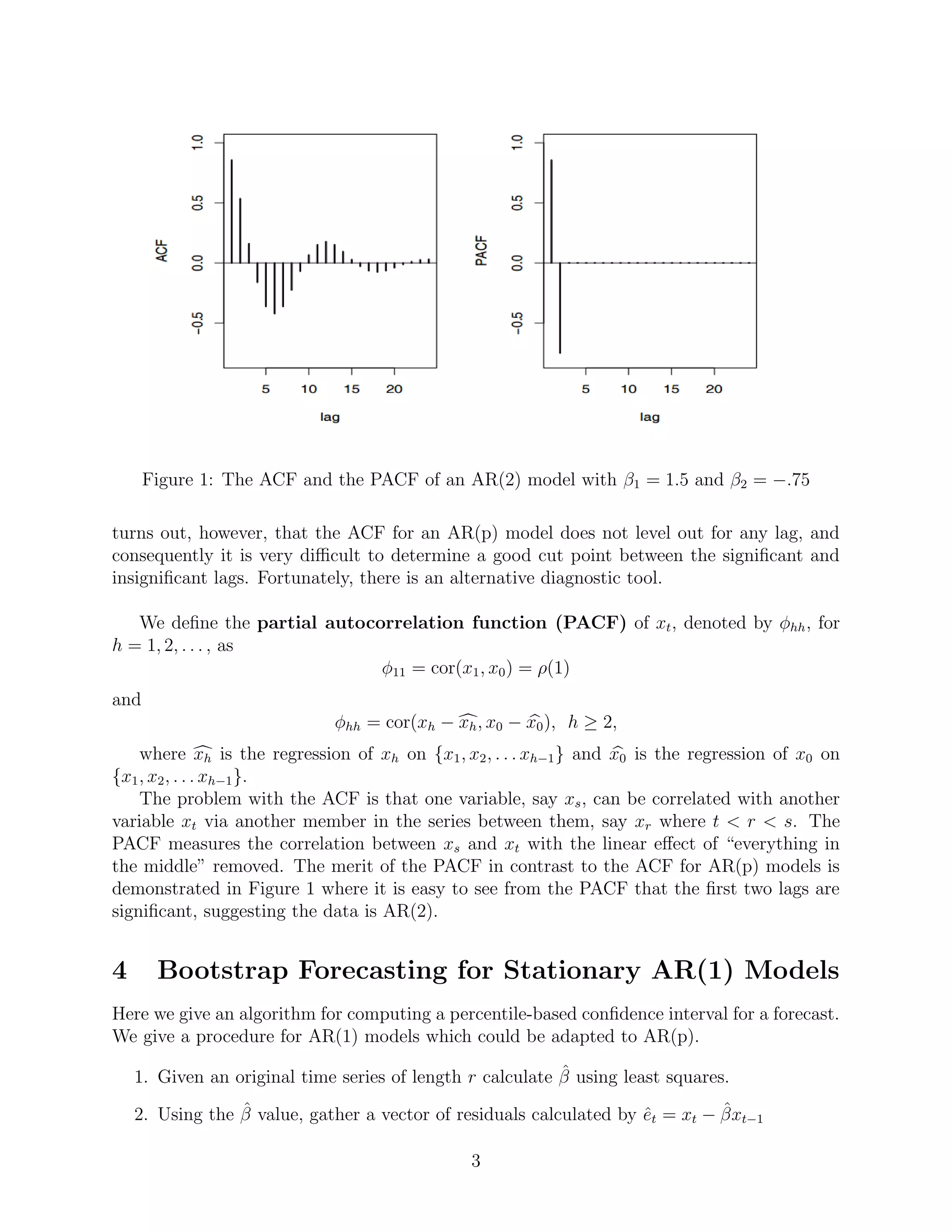
9. While the plot does display a pattern, we notice that the correlations are small. We conclude
that the assumption of no correlation is reasonable in this case.
5 10 15 20 25
-0.10.00.10.20.3
Lag (Quarters)
PACF
Figure 5: PACF of Estimated Residuals
6.2 A Bootstrap Confidence Interval
Next, we estimate a forecast confidence interval using bootstrap. The workhorse function
here is tsboot from the boot package in R. We use this to perform the procedure described
in Section 4. After generating 1000 bootstrap time series we obtain the following:
ˆβ .362
Forecast growth rate 0.00795
Forecast Growth Rate CI (0.00011, 0.01564)
Forecast CI (dollars) (16625.08, 16885.17)
Based on this estimate we expect GNP in 2016 Q2 to be between about $16,625 and
$16,885.
We notice that the bootstrap forecast for the growth rate, .8% growth differs somewhat
from the parametric estimate of .5% growth and that the bootstrap confidence interval for
GNP in 2016 Q2 is wider than the parametric interval.
In addition, we can estimate the variance of an OLS estimate of β by looking at the
variance of the 1000 bootstrap estimates. We find that Var(ˆβ) = .002921 which closely
matches the theoretical value described above.
References
[1] Chernick, Michael R. Robert A. LaBudde, An Introduction To Bootstrap Methods with Applications to
R John Wiley and Sons 2012.
[2] Cryer,Jonathan D., Kung-Sik Chan, Time Series Analysis: With Applications in R Springer, Second Ed.
2008. pp 160-161.
8

10. [3] Shumway, Robert H., David S. Stover, Time Series Analysis and Applications With R Examples, EZ
Green Edition 2016.4, 2016.
[4] Real Gross National Product [GNPC96],US. Bureau of Economic Analysis, retrieved from FRED, Federal
Reserve Bank of St. Louis <https://research.stlouisfed.org/fred2/series/GNPC96>, June 9, 2016.
9